Content from Intro to Raster Data
Last updated on 2024-10-15 | Edit this page
Overview
Questions
- What is a raster dataset?
- How do I work with and plot raster data in R?
- How can I handle missing or bad data values for a raster?
Objectives
- Describe the fundamental attributes of a raster dataset.
- Explore raster attributes and metadata using R.
- Import rasters into R using the
terrapackage. - Plot a raster file in R using the
ggplot2package. - Describe the difference between single- and multi-band rasters.
Things You’ll Need To Complete This Episode
See the lesson homepage for detailed information about the software, data, and other prerequisites you will need to work through the examples in this episode.
In this episode, we will introduce the fundamental principles, packages and metadata/raster attributes that are needed to work with raster data in R. We will discuss some of the core metadata elements that we need to understand to work with rasters in R, including CRS and resolution. We will also explore missing and bad data values as stored in a raster and how R handles these elements.
We will continue to work with the dplyr and
ggplot2 packages that were introduced in the Introduction to R
for Geospatial Data lesson. We will use two additional packages in
this episode to work with raster data - the terra and
sf packages. Make sure that you have these packages
loaded.
R
library(terra)
library(ggplot2)
library(dplyr)
Introduce the Data
If not already discussed, introduce the datasets that will be used in this lesson. A brief introduction to the datasets can be found on the Geospatial workshop homepage.
For more detailed information about the datasets, check out the Geospatial workshop data page.
View Raster File Attributes
We will be working with a series of GeoTIFF files in this lesson. The
GeoTIFF format contains a set of embedded tags with metadata about the
raster data. We can use the function describe() to get
information about our raster data before we read that data into R. It is
ideal to do this before importing your data.
R
describe("data/NEON-DS-Airborne-Remote-Sensing/HARV/DSM/HARV_dsmCrop.tif")
OUTPUT
 [1] "Driver: GTiff/GeoTIFF"
 [2] "Files: data/NEON-DS-Airborne-Remote-Sensing/HARV/DSM/HARV_dsmCrop.tif"
 [3] "Size is 1697, 1367"
 [4] "Coordinate System is:"
 [5] "PROJCRS[\"WGS 84 / UTM zone 18N\","
 [6] "    BASEGEOGCRS[\"WGS 84\","
 [7] "        DATUM[\"World Geodetic System 1984\","
 [8] "            ELLIPSOID[\"WGS 84\",6378137,298.257223563,"
 [9] "                LENGTHUNIT[\"metre\",1]]],"
[10] "        PRIMEM[\"Greenwich\",0,"
[11] "            ANGLEUNIT[\"degree\",0.0174532925199433]],"
[12] "        ID[\"EPSG\",4326]],"
[13] "    CONVERSION[\"UTM zone 18N\","
[14] "        METHOD[\"Transverse Mercator\","
[15] "            ID[\"EPSG\",9807]],"
[16] "        PARAMETER[\"Latitude of natural origin\",0,"
[17] "            ANGLEUNIT[\"degree\",0.0174532925199433],"
[18] "            ID[\"EPSG\",8801]],"
[19] "        PARAMETER[\"Longitude of natural origin\",-75,"
[20] "            ANGLEUNIT[\"degree\",0.0174532925199433],"
[21] "            ID[\"EPSG\",8802]],"
[22] "        PARAMETER[\"Scale factor at natural origin\",0.9996,"
[23] "            SCALEUNIT[\"unity\",1],"
[24] "            ID[\"EPSG\",8805]],"
[25] "        PARAMETER[\"False easting\",500000,"
[26] "            LENGTHUNIT[\"metre\",1],"
[27] "            ID[\"EPSG\",8806]],"
[28] "        PARAMETER[\"False northing\",0,"
[29] "            LENGTHUNIT[\"metre\",1],"
[30] "            ID[\"EPSG\",8807]]],"
[31] "    CS[Cartesian,2],"
[32] "        AXIS[\"(E)\",east,"
[33] "            ORDER[1],"
[34] "            LENGTHUNIT[\"metre\",1]],"
[35] "        AXIS[\"(N)\",north,"
[36] "            ORDER[2],"
[37] "            LENGTHUNIT[\"metre\",1]],"
[38] "    USAGE["
[39] "        SCOPE[\"Engineering survey, topographic mapping.\"],"
[40] "        AREA[\"Between 78°W and 72°W, northern hemisphere between equator and 84°N, onshore and offshore. Bahamas. Canada - Nunavut; Ontario; Quebec. Colombia. Cuba. Ecuador. Greenland. Haiti. Jamica. Panama. Turks and Caicos Islands. United States (USA). Venezuela.\"],"
[41] "        BBOX[0,-78,84,-72]],"
[42] "    ID[\"EPSG\",32618]]"
[43] "Data axis to CRS axis mapping: 1,2"
[44] "Origin = (731453.000000000000000,4713838.000000000000000)"
[45] "Pixel Size = (1.000000000000000,-1.000000000000000)"
[46] "Metadata:"
[47] "  AREA_OR_POINT=Area"
[48] "Image Structure Metadata:"
[49] "  COMPRESSION=LZW"
[50] "  INTERLEAVE=BAND"
[51] "Corner Coordinates:"
[52] "Upper Left  (  731453.000, 4713838.000) ( 72d10'52.71\"W, 42d32'32.18\"N)"
[53] "Lower Left  (  731453.000, 4712471.000) ( 72d10'54.71\"W, 42d31'47.92\"N)"
[54] "Upper Right (  733150.000, 4713838.000) ( 72d 9'38.40\"W, 42d32'30.35\"N)"
[55] "Lower Right (  733150.000, 4712471.000) ( 72d 9'40.41\"W, 42d31'46.08\"N)"
[56] "Center      (  732301.500, 4713154.500) ( 72d10'16.56\"W, 42d32' 9.13\"N)"
[57] "Band 1 Block=1697x1 Type=Float64, ColorInterp=Gray"
[58] "  Min=305.070 Max=416.070 "
[59] "  Minimum=305.070, Maximum=416.070, Mean=359.853, StdDev=17.832"
[60] "  NoData Value=-9999"
[61] "  Metadata:"
[62] "    STATISTICS_MAXIMUM=416.06997680664"
[63] "    STATISTICS_MEAN=359.85311802914"
[64] "    STATISTICS_MINIMUM=305.07000732422"
[65] "    STATISTICS_STDDEV=17.83169335933"
If you wish to store this information in R, you can do the following:
R
HARV_dsmCrop_info <- capture.output(
  describe("data/NEON-DS-Airborne-Remote-Sensing/HARV/DSM/HARV_dsmCrop.tif")
)
Each line of text that was printed to the console is now stored as an
element of the character vector HARV_dsmCrop_info. We will
be exploring this data throughout this episode. By the end of this
episode, you will be able to explain and understand the output
above.
Open a Raster in R
Now that we’ve previewed the metadata for our GeoTIFF, let’s import
this raster dataset into R and explore its metadata more closely. We can
use the rast() function to open a raster in R.
Data Tip - Object names
To improve code readability, file and object names should be used
that make it clear what is in the file. The data for this episode were
collected from Harvard Forest so we’ll use a naming convention of
datatype_HARV.
First we will load our raster file into R and view the data structure.
R
DSM_HARV <-
  rast("data/NEON-DS-Airborne-Remote-Sensing/HARV/DSM/HARV_dsmCrop.tif")

DSM_HARV
OUTPUT
class       : SpatRaster
dimensions  : 1367, 1697, 1  (nrow, ncol, nlyr)
resolution  : 1, 1  (x, y)
extent      : 731453, 733150, 4712471, 4713838  (xmin, xmax, ymin, ymax)
coord. ref. : WGS 84 / UTM zone 18N (EPSG:32618)
source      : HARV_dsmCrop.tif
name        : HARV_dsmCrop
min value   :       305.07
max value   :       416.07
The information above includes a report of min and max values, but no other data range statistics. Similar to other R data structures like vectors and data frame columns, descriptive statistics for raster data can be retrieved like
R
summary(DSM_HARV)
WARNING
Warning: [summary] used a sampleOUTPUT
  HARV_dsmCrop
 Min.   :305.6
 1st Qu.:345.6
 Median :359.6
 Mean   :359.8
 3rd Qu.:374.3
 Max.   :414.7
but note the warning - unless you force R to calculate these
statistics using every cell in the raster, it will take a random sample
of 100,000 cells and calculate from that instead. To force calculation
all the values, you can use the function values:
R
summary(values(DSM_HARV))
OUTPUT
  HARV_dsmCrop
 Min.   :305.1
 1st Qu.:345.6
 Median :359.7
 Mean   :359.9
 3rd Qu.:374.3
 Max.   :416.1
To visualise this data in R using ggplot2, we need to
convert it to a dataframe. We learned about dataframes in an
earlier lesson. The terra package has an built-in
function for conversion to a plotable dataframe.
R
DSM_HARV_df <- as.data.frame(DSM_HARV, xy = TRUE)
Now when we view the structure of our data, we will see a standard dataframe format.
R
str(DSM_HARV_df)
OUTPUT
'data.frame': 2319799 obs. of 3 variables:
$ x : num 731454 731454 731456 731456 731458 ...
$ y : num 4713838 4713838 4713838 4713838 4713838 ...
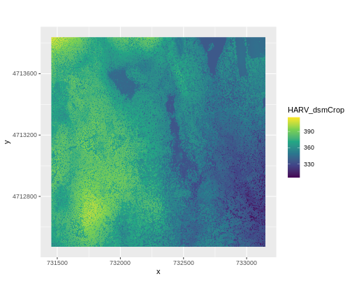
$ HARV_dsmCrop: num 409 408 407 407 409 ...We can use ggplot() to plot this data. We will set the
color scale to scale_fill_viridis_c which is a
color-blindness friendly color scale. We will also use the
coord_quickmap() function to use an approximate Mercator
projection for our plots. This approximation is suitable for small areas
that are not too close to the poles. Other coordinate systems are
available in ggplot2 if needed, you can learn about them at their help
page ?coord_map.
R
ggplot() +
    geom_raster(data = DSM_HARV_df , aes(x = x, y = y, fill = HARV_dsmCrop)) +
    scale_fill_viridis_c() +
    coord_quickmap()
Plotting Tip
More information about the Viridis palette used above at R Viridis package documentation.
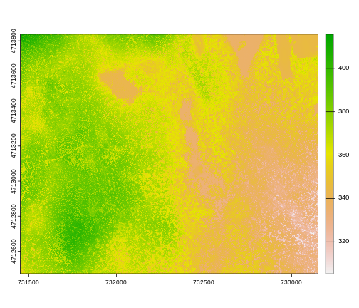
Plotting Tip
For faster, simpler plots, you can use the plot function
from the terra package.
See ?plot for more arguments to customize the plot
R
plot(DSM_HARV)
This map shows the elevation of our study site in Harvard Forest. From the legend, we can see that the maximum elevation is ~400, but we can’t tell whether this is 400 feet or 400 meters because the legend doesn’t show us the units. We can look at the metadata of our object to see what the units are. Much of the metadata that we’re interested in is part of the CRS. We introduced the concept of a CRS in an earlier lesson.
Now we will see how features of the CRS appear in our data file and what meanings they have.
View Raster Coordinate Reference System (CRS) in R
We can view the CRS string associated with our R object using
thecrs() function.
R
crs(DSM_HARV, proj = TRUE)
OUTPUT
[1] "+proj=utm +zone=18 +datum=WGS84 +units=m +no_defs"Challenge
What units are our data in?
+units=m tells us that our data is in meters.
Understanding CRS in Proj4 Format
The CRS for our data is given to us by R in proj4
format. Let’s break down the pieces of proj4 string. The
string contains all of the individual CRS elements that R or another GIS
might need. Each element is specified with a + sign,
similar to how a .csv file is delimited or broken up by a
,. After each + we see the CRS element being
defined. For example projection (proj=) and datum
(datum=).
UTM Proj4 String
A projection string (like the one of DSM_HARV) specifies
the UTM projection as follows:
+proj=utm +zone=18 +datum=WGS84 +units=m +no_defs +ellps=WGS84 +towgs84=0,0,0
- proj=utm: the projection is UTM, UTM has several zones.
- zone=18: the zone is 18
- datum=WGS84: the datum is WGS84 (the datum refers to the 0,0 reference for the coordinate system used in the projection)
- units=m: the units for the coordinates are in meters
- ellps=WGS84: the ellipsoid (how the earth’s roundness is calculated) for the data is WGS84
Note that the zone is unique to the UTM projection. Not all CRSs will have a zone. Image source: Chrismurf at English Wikipedia, via Wikimedia Commons (CC-BY).

Calculate Raster Min and Max Values
It is useful to know the minimum or maximum values of a raster dataset. In this case, given we are working with elevation data, these values represent the min/max elevation range at our site.
Raster statistics are often calculated and embedded in a GeoTIFF for us. We can view these values:
R
minmax(DSM_HARV)
OUTPUT
    HARV_dsmCrop
min       305.07
max       416.07
R
min(values(DSM_HARV))
OUTPUT
[1] 305.07R
max(values(DSM_HARV))
OUTPUT
[1] 416.07Data Tip - Set min and max values
If the minimum and maximum values haven’t already been calculated, we
can calculate them using the setMinMax() function.
R
DSM_HARV <- setMinMax(DSM_HARV)
We can see that the elevation at our site ranges from 305.0700073m to 416.0699768m.
Raster Bands
The Digital Surface Model object (DSM_HARV) that we’ve
been working with is a single band raster. This means that there is only
one dataset stored in the raster: surface elevation in meters for one
time period.
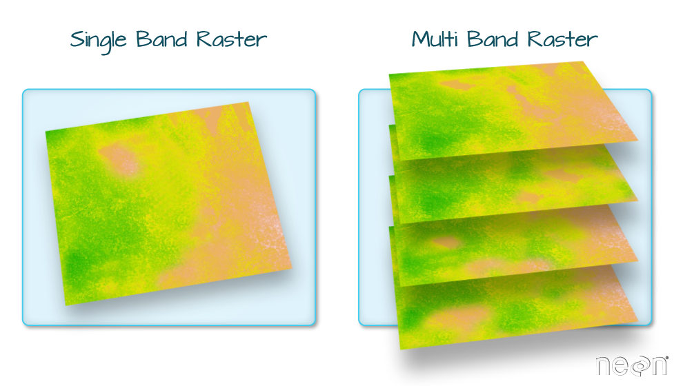
A raster dataset can contain one or more bands. We can use the
rast() function to import one single band from a single or
multi-band raster. We can view the number of bands in a raster using the
nlyr() function.
R
nlyr(DSM_HARV)
OUTPUT
[1] 1However, raster data can also be multi-band, meaning that one raster file contains data for more than one variable or time period for each cell. Jump to a later episode in this series for information on working with multi-band rasters: Work with Multi-band Rasters in R.
Dealing with Missing Data
Raster data often has a NoDataValue associated with it.
This is a value assigned to pixels where data is missing or no data were
collected.
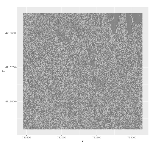
By default the shape of a raster is always rectangular. So if we have
a dataset that has a shape that isn’t rectangular, some pixels at the
edge of the raster will have NoDataValues. This often
happens when the data were collected by an airplane which only flew over
some part of a defined region.
In the image below, the pixels that are black have
NoDataValues. The camera did not collect data in these
areas.
In the next image, the black edges have been assigned
NoDataValue. R doesn’t render pixels that contain a
specified NoDataValue. R assigns missing data with the
NoDataValue as NA.
The difference here shows up as ragged edges on the plot, rather than black spaces where there is no data.
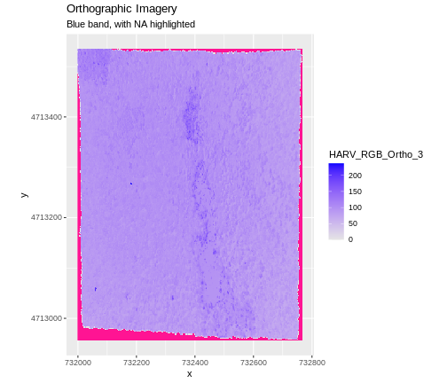
If your raster already has NA values set correctly but
you aren’t sure where they are, you can deliberately plot them in a
particular colour. This can be useful when checking a dataset’s
coverage. For instance, sometimes data can be missing where a sensor
could not ‘see’ its target data, and you may wish to locate that missing
data and fill it in.
To highlight NA values in ggplot, alter the
scale_fill_*() layer to contain a colour instruction for
NA values, like
scale_fill_viridis_c(na.value = 'deeppink')
The value that is conventionally used to take note of missing data
(the NoDataValue value) varies by the raster data type. For
floating-point rasters, the figure -3.4e+38 is a common
default, and for integers, -9999 is common. Some
disciplines have specific conventions that vary from these common
values.
In some cases, other NA values may be more appropriate.
An NA value should be a) outside the range of valid values,
and b) a value that fits the data type in use. For instance, if your
data ranges continuously from -20 to 100, 0 is not an acceptable
NA value! Or, for categories that number 1-15, 0 might be
fine for NA, but using -.000003 will force you to save the
GeoTIFF on disk as a floating point raster, resulting in a bigger
file.
If we are lucky, our GeoTIFF file has a tag that tells us what is the
NoDataValue. If we are less lucky, we can find that
information in the raster’s metadata. If a NoDataValue was
stored in the GeoTIFF tag, when R opens up the raster, it will assign
each instance of the value to NA. Values of NA
will be ignored by R as demonstrated above.
Challenge
Use the output from the describe() and
sources() functions to find out what
NoDataValue is used for our DSM_HARV
dataset.
R
describe(sources(DSM_HARV))
OUTPUT
 [1] "Driver: GTiff/GeoTIFF"
 [2] "Files: /home/runner/work/r-raster-vector-geospatial/r-raster-vector-geospatial/site/built/data/NEON-DS-Airborne-Remote-Sensing/HARV/DSM/HARV_dsmCrop.tif"
 [3] "Size is 1697, 1367"
 [4] "Coordinate System is:"
 [5] "PROJCRS[\"WGS 84 / UTM zone 18N\","
 [6] "    BASEGEOGCRS[\"WGS 84\","
 [7] "        DATUM[\"World Geodetic System 1984\","
 [8] "            ELLIPSOID[\"WGS 84\",6378137,298.257223563,"
 [9] "                LENGTHUNIT[\"metre\",1]]],"
[10] "        PRIMEM[\"Greenwich\",0,"
[11] "            ANGLEUNIT[\"degree\",0.0174532925199433]],"
[12] "        ID[\"EPSG\",4326]],"
[13] "    CONVERSION[\"UTM zone 18N\","
[14] "        METHOD[\"Transverse Mercator\","
[15] "            ID[\"EPSG\",9807]],"
[16] "        PARAMETER[\"Latitude of natural origin\",0,"
[17] "            ANGLEUNIT[\"degree\",0.0174532925199433],"
[18] "            ID[\"EPSG\",8801]],"
[19] "        PARAMETER[\"Longitude of natural origin\",-75,"
[20] "            ANGLEUNIT[\"degree\",0.0174532925199433],"
[21] "            ID[\"EPSG\",8802]],"
[22] "        PARAMETER[\"Scale factor at natural origin\",0.9996,"
[23] "            SCALEUNIT[\"unity\",1],"
[24] "            ID[\"EPSG\",8805]],"
[25] "        PARAMETER[\"False easting\",500000,"
[26] "            LENGTHUNIT[\"metre\",1],"
[27] "            ID[\"EPSG\",8806]],"
[28] "        PARAMETER[\"False northing\",0,"
[29] "            LENGTHUNIT[\"metre\",1],"
[30] "            ID[\"EPSG\",8807]]],"
[31] "    CS[Cartesian,2],"
[32] "        AXIS[\"(E)\",east,"
[33] "            ORDER[1],"
[34] "            LENGTHUNIT[\"metre\",1]],"
[35] "        AXIS[\"(N)\",north,"
[36] "            ORDER[2],"
[37] "            LENGTHUNIT[\"metre\",1]],"
[38] "    USAGE["
[39] "        SCOPE[\"Engineering survey, topographic mapping.\"],"
[40] "        AREA[\"Between 78°W and 72°W, northern hemisphere between equator and 84°N, onshore and offshore. Bahamas. Canada - Nunavut; Ontario; Quebec. Colombia. Cuba. Ecuador. Greenland. Haiti. Jamica. Panama. Turks and Caicos Islands. United States (USA). Venezuela.\"],"
[41] "        BBOX[0,-78,84,-72]],"
[42] "    ID[\"EPSG\",32618]]"
[43] "Data axis to CRS axis mapping: 1,2"
[44] "Origin = (731453.000000000000000,4713838.000000000000000)"
[45] "Pixel Size = (1.000000000000000,-1.000000000000000)"
[46] "Metadata:"
[47] "  AREA_OR_POINT=Area"
[48] "Image Structure Metadata:"
[49] "  COMPRESSION=LZW"
[50] "  INTERLEAVE=BAND"
[51] "Corner Coordinates:"
[52] "Upper Left  (  731453.000, 4713838.000) ( 72d10'52.71\"W, 42d32'32.18\"N)"
[53] "Lower Left  (  731453.000, 4712471.000) ( 72d10'54.71\"W, 42d31'47.92\"N)"
[54] "Upper Right (  733150.000, 4713838.000) ( 72d 9'38.40\"W, 42d32'30.35\"N)"
[55] "Lower Right (  733150.000, 4712471.000) ( 72d 9'40.41\"W, 42d31'46.08\"N)"
[56] "Center      (  732301.500, 4713154.500) ( 72d10'16.56\"W, 42d32' 9.13\"N)"
[57] "Band 1 Block=1697x1 Type=Float64, ColorInterp=Gray"
[58] "  Min=305.070 Max=416.070 "
[59] "  Minimum=305.070, Maximum=416.070, Mean=359.853, StdDev=17.832"
[60] "  NoData Value=-9999"
[61] "  Metadata:"
[62] "    STATISTICS_MAXIMUM=416.06997680664"
[63] "    STATISTICS_MEAN=359.85311802914"
[64] "    STATISTICS_MINIMUM=305.07000732422"
[65] "    STATISTICS_STDDEV=17.83169335933"
NoDataValue are encoded as -9999.
Bad Data Values in Rasters
Bad data values are different from NoDataValues. Bad
data values are values that fall outside of the applicable range of a
dataset.
Examples of Bad Data Values:
- The normalized difference vegetation index (NDVI), which is a measure of greenness, has a valid range of -1 to 1. Any value outside of that range would be considered a “bad” or miscalculated value.
- Reflectance data in an image will often range from 0-1 or 0-10,000 depending upon how the data are scaled. Thus a value greater than 1 or greater than 10,000 is likely caused by an error in either data collection or processing.
Find Bad Data Values
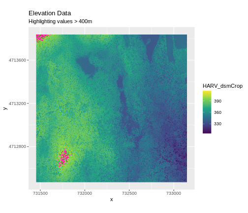
Sometimes a raster’s metadata will tell us the range of expected values for a raster. Values outside of this range are suspect and we need to consider that when we analyze the data. Sometimes, we need to use some common sense and scientific insight as we examine the data - just as we would for field data to identify questionable values.
Plotting data with appropriate highlighting can help reveal patterns in bad values and may suggest a solution. Below, reclassification is used to highlight elevation values over 400m with a contrasting colour.
Create A Histogram of Raster Values
We can explore the distribution of values contained within our raster
using the geom_histogram() function which produces a
histogram. Histograms are often useful in identifying outliers and bad
data values in our raster data.
R
ggplot() +
    geom_histogram(data = DSM_HARV_df, aes(HARV_dsmCrop))
OUTPUT
`stat_bin()` using `bins = 30`. Pick better value with `binwidth`.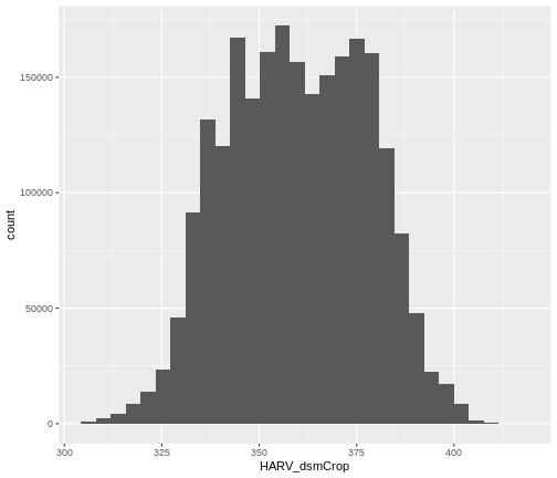
Notice that a warning message is thrown when R creates the histogram.
stat_bin() using bins = 30. Pick better
value with binwidth.
This warning is caused by a default setting in
geom_histogram enforcing that there are 30 bins for the
data. We can define the number of bins we want in the histogram by using
the bins value in the geom_histogram()
function.
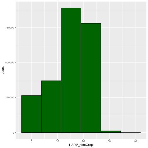
R
ggplot() +
    geom_histogram(data = DSM_HARV_df, aes(HARV_dsmCrop), bins = 40)
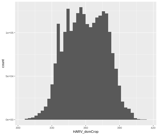
Note that the shape of this histogram looks similar to the previous
one that was created using the default of 30 bins. The distribution of
elevation values for our Digital Surface Model (DSM) looks
reasonable. It is likely there are no bad data values in this particular
raster.
Challenge: Explore Raster Metadata
Use describe() to determine the following about the
NEON-DS-Airborne-Remote-Sensing/HARV/DSM/HARV_DSMhill.tif
file:
- Does this file have the same CRS as
DSM_HARV? - What is the
NoDataValue? - What is resolution of the raster data?
- How large would a 5x5 pixel area be on the Earth’s surface?
- Is the file a multi- or single-band raster?
Notice: this file is a hillshade. We will learn about hillshades in the Working with Multi-band Rasters in R episode.
R
describe("data/NEON-DS-Airborne-Remote-Sensing/HARV/DSM/HARV_DSMhill.tif")
OUTPUT
 [1] "Driver: GTiff/GeoTIFF"
 [2] "Files: data/NEON-DS-Airborne-Remote-Sensing/HARV/DSM/HARV_DSMhill.tif"
 [3] "Size is 1697, 1367"
 [4] "Coordinate System is:"
 [5] "PROJCRS[\"WGS 84 / UTM zone 18N\","
 [6] "    BASEGEOGCRS[\"WGS 84\","
 [7] "        DATUM[\"World Geodetic System 1984\","
 [8] "            ELLIPSOID[\"WGS 84\",6378137,298.257223563,"
 [9] "                LENGTHUNIT[\"metre\",1]]],"
[10] "        PRIMEM[\"Greenwich\",0,"
[11] "            ANGLEUNIT[\"degree\",0.0174532925199433]],"
[12] "        ID[\"EPSG\",4326]],"
[13] "    CONVERSION[\"UTM zone 18N\","
[14] "        METHOD[\"Transverse Mercator\","
[15] "            ID[\"EPSG\",9807]],"
[16] "        PARAMETER[\"Latitude of natural origin\",0,"
[17] "            ANGLEUNIT[\"degree\",0.0174532925199433],"
[18] "            ID[\"EPSG\",8801]],"
[19] "        PARAMETER[\"Longitude of natural origin\",-75,"
[20] "            ANGLEUNIT[\"degree\",0.0174532925199433],"
[21] "            ID[\"EPSG\",8802]],"
[22] "        PARAMETER[\"Scale factor at natural origin\",0.9996,"
[23] "            SCALEUNIT[\"unity\",1],"
[24] "            ID[\"EPSG\",8805]],"
[25] "        PARAMETER[\"False easting\",500000,"
[26] "            LENGTHUNIT[\"metre\",1],"
[27] "            ID[\"EPSG\",8806]],"
[28] "        PARAMETER[\"False northing\",0,"
[29] "            LENGTHUNIT[\"metre\",1],"
[30] "            ID[\"EPSG\",8807]]],"
[31] "    CS[Cartesian,2],"
[32] "        AXIS[\"(E)\",east,"
[33] "            ORDER[1],"
[34] "            LENGTHUNIT[\"metre\",1]],"
[35] "        AXIS[\"(N)\",north,"
[36] "            ORDER[2],"
[37] "            LENGTHUNIT[\"metre\",1]],"
[38] "    USAGE["
[39] "        SCOPE[\"Engineering survey, topographic mapping.\"],"
[40] "        AREA[\"Between 78°W and 72°W, northern hemisphere between equator and 84°N, onshore and offshore. Bahamas. Canada - Nunavut; Ontario; Quebec. Colombia. Cuba. Ecuador. Greenland. Haiti. Jamica. Panama. Turks and Caicos Islands. United States (USA). Venezuela.\"],"
[41] "        BBOX[0,-78,84,-72]],"
[42] "    ID[\"EPSG\",32618]]"
[43] "Data axis to CRS axis mapping: 1,2"
[44] "Origin = (731453.000000000000000,4713838.000000000000000)"
[45] "Pixel Size = (1.000000000000000,-1.000000000000000)"
[46] "Metadata:"
[47] "  AREA_OR_POINT=Area"
[48] "Image Structure Metadata:"
[49] "  COMPRESSION=LZW"
[50] "  INTERLEAVE=BAND"
[51] "Corner Coordinates:"
[52] "Upper Left  (  731453.000, 4713838.000) ( 72d10'52.71\"W, 42d32'32.18\"N)"
[53] "Lower Left  (  731453.000, 4712471.000) ( 72d10'54.71\"W, 42d31'47.92\"N)"
[54] "Upper Right (  733150.000, 4713838.000) ( 72d 9'38.40\"W, 42d32'30.35\"N)"
[55] "Lower Right (  733150.000, 4712471.000) ( 72d 9'40.41\"W, 42d31'46.08\"N)"
[56] "Center      (  732301.500, 4713154.500) ( 72d10'16.56\"W, 42d32' 9.13\"N)"
[57] "Band 1 Block=1697x1 Type=Float64, ColorInterp=Gray"
[58] "  Min=-0.714 Max=1.000 "
[59] "  Minimum=-0.714, Maximum=1.000, Mean=0.313, StdDev=0.481"
[60] "  NoData Value=-9999"
[61] "  Metadata:"
[62] "    STATISTICS_MAXIMUM=0.99999973665016"
[63] "    STATISTICS_MEAN=0.31255246777216"
[64] "    STATISTICS_MINIMUM=-0.71362979358008"
[65] " STATISTICS_STDDEV=0.48129385401108" - If this file has the same CRS as DSM_HARV? Yes: UTM Zone 18, WGS84, meters.
- What format
NoDataValuestake? -9999 - The resolution of the raster data? 1x1
- How large a 5x5 pixel area would be? 5mx5m How? We are given resolution of 1x1 and units in meters, therefore resolution of 5x5 means 5x5m.
- Is the file a multi- or single-band raster? Single.
More Resources
Key Points
- The GeoTIFF file format includes metadata about the raster data.
- To plot raster data with the
ggplot2package, we need to convert it to a dataframe. - R stores CRS information in the Proj4 format.
- Be careful when dealing with missing or bad data values.
Content from Plot Raster Data
Last updated on 2024-10-15 | Edit this page
Overview
Questions
- How can I create categorized or customized maps of raster data?
- How can I customize the color scheme of a raster image?
- How can I layer raster data in a single image?
Objectives
- Build customized plots for a single band raster using the
ggplot2package. - Layer a raster dataset on top of a hillshade to create an elegant basemap.
Things You’ll Need To Complete This Episode
See the lesson homepage for detailed information about the software, data, and other prerequisites you will need to work through the examples in this episode.
Plot Raster Data in R
This episode covers how to plot a raster in R using the
ggplot2 package with customized coloring schemes. It also
covers how to layer a raster on top of a hillshade to produce an
eloquent map. We will continue working with the Digital Surface Model
(DSM) raster for the NEON Harvard Forest Field Site.
Plotting Data Using Breaks
In the previous episode, we viewed our data using a continuous color
ramp. For clarity and visibility of the plot, we may prefer to view the
data “symbolized” or colored according to ranges of values. This is
comparable to a “classified” map. To do this, we need to tell
ggplot how many groups to break our data into, and where
those breaks should be. To make these decisions, it is useful to first
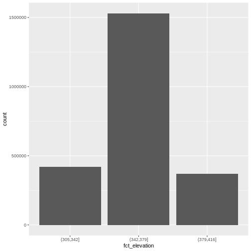
explore the distribution of the data using a bar plot. To begin with, we
will use dplyr’s mutate() function combined
with cut() to split the data into 3 bins.
R
DSM_HARV_df <- DSM_HARV_df %>%
                mutate(fct_elevation = cut(HARV_dsmCrop, breaks = 3))

ggplot() +
    geom_bar(data = DSM_HARV_df, aes(fct_elevation))
If we want to know the cutoff values for the groups, we can ask for
the unique values of fct_elevation:
R
unique(DSM_HARV_df$fct_elevation)
OUTPUT
[1] (379,416] (342,379] (305,342]
Levels: (305,342] (342,379] (379,416]
And we can get the count of values in each group using
dplyr’s count() function:
R
DSM_HARV_df %>%
        count(fct_elevation)
OUTPUT
  fct_elevation       n
1     (305,342]  418891
2     (342,379] 1530073
3     (379,416]  370835
We might prefer to customize the cutoff values for these groups. Lets
round the cutoff values so that we have groups for the ranges of 301–350
m, 351–400 m, and 401–450 m. To implement this we will give
mutate() a numeric vector of break points instead of the
number of breaks we want.
R
custom_bins <- c(300, 350, 400, 450)

DSM_HARV_df <- DSM_HARV_df %>%
  mutate(fct_elevation_2 = cut(HARV_dsmCrop, breaks = custom_bins))

unique(DSM_HARV_df$fct_elevation_2)
OUTPUT
[1] (400,450] (350,400] (300,350]
Levels: (300,350] (350,400] (400,450]
Data Tips
Note that when we assign break values a set of 4 values will result in 3 bins of data.
The bin intervals are shown using ( to mean exclusive
and ] to mean inclusive. For example:
(305, 342] means “from 306 through 342”.
And now we can plot our bar plot again, using the new groups:
R
ggplot() +
  geom_bar(data = DSM_HARV_df, aes(fct_elevation_2))
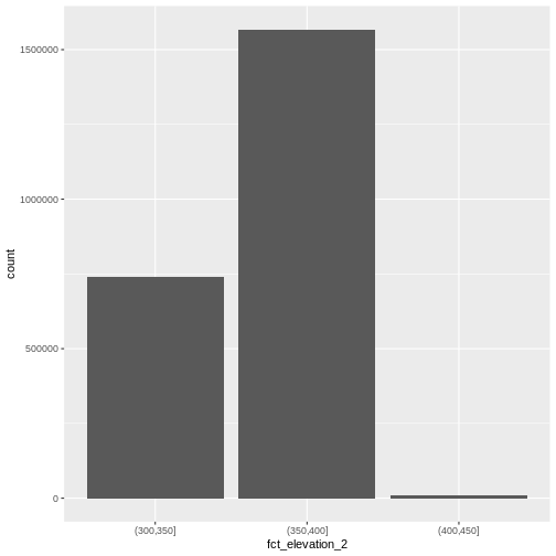
And we can get the count of values in each group in the same way we did before:
R
DSM_HARV_df %>%
  count(fct_elevation_2)
OUTPUT
fct_elevation_2 n
1 (300,350] 741815
2 (350,400] 1567316
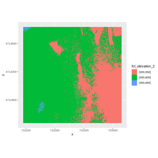
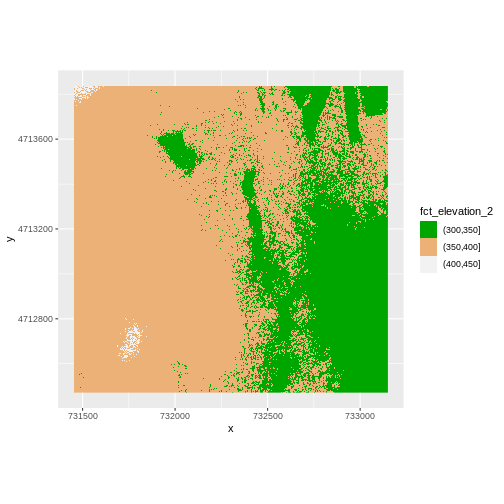
3 (400,450] 10668We can use those groups to plot our raster data, with each group being a different color:
R
ggplot() +
  geom_raster(data = DSM_HARV_df , aes(x = x, y = y, fill = fct_elevation_2)) +
  coord_quickmap()
The plot above uses the default colors inside ggplot for
raster objects. We can specify our own colors to make the plot look a
little nicer. R has a built in set of colors for plotting terrain, which
are built in to the terrain.colors() function. Since we
have three bins, we want to create a 3-color palette:
R
terrain.colors(3)
OUTPUT
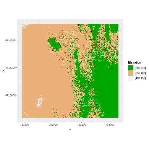
[1] "#00A600" "#ECB176" "#F2F2F2"The terrain.colors() function returns hex
colors - each of these character strings represents a color. To use
these in our map, we pass them across using the
scale_fill_manual() function.
R
ggplot() +
 geom_raster(data = DSM_HARV_df , aes(x = x, y = y,
                                      fill = fct_elevation_2)) +
    scale_fill_manual(values = terrain.colors(3)) +
    coord_quickmap()
More Plot Formatting
If we need to create multiple plots using the same color palette, we
can create an R object (my_col) for the set of colors that
we want to use. We can then quickly change the palette across all plots
by modifying the my_col object, rather than each individual
plot.
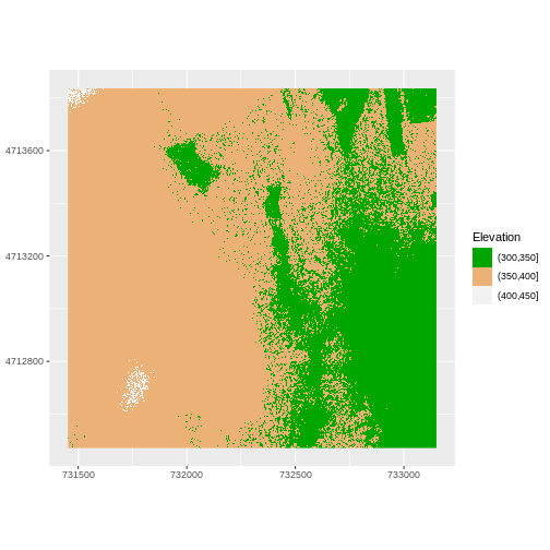
We can label the x- and y-axes of our plot too using
xlab and ylab. We can also give the legend a
more meaningful title by passing a value to the name
argument of the scale_fill_manual() function.
R
my_col <- terrain.colors(3)

ggplot() +
 geom_raster(data = DSM_HARV_df , aes(x = x, y = y,
                                      fill = fct_elevation_2)) +
    scale_fill_manual(values = my_col, name = "Elevation") +
    coord_quickmap()
Or we can also turn off the labels of both axes by passing
element_blank() to the relevant part of the
theme() function.
R
ggplot() +
 geom_raster(data = DSM_HARV_df , aes(x = x, y = y,
                                      fill = fct_elevation_2)) +
    scale_fill_manual(values = my_col, name = "Elevation") +
    theme(axis.title = element_blank()) +
    coord_quickmap()
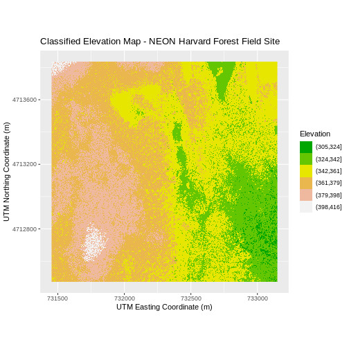
Challenge: Plot Using Custom Breaks
Create a plot of the Harvard Forest Digital Surface Model (DSM) that has:
- Six classified ranges of values (break points) that are evenly divided among the range of pixel values.
- Axis labels.
- A plot title.
R
DSM_HARV_df <- DSM_HARV_df  %>%
               mutate(fct_elevation_6 = cut(HARV_dsmCrop, breaks = 6))

 my_col <- terrain.colors(6)

ggplot() +
    geom_raster(data = DSM_HARV_df , aes(x = x, y = y,
                                      fill = fct_elevation_6)) +
    scale_fill_manual(values = my_col, name = "Elevation") +
    ggtitle("Classified Elevation Map - NEON Harvard Forest Field Site") +
    xlab("UTM Easting Coordinate (m)") +
    ylab("UTM Northing Coordinate (m)") +
    coord_quickmap()
Layering Rasters
We can layer a raster on top of a hillshade raster for the same area, and use a transparency factor to create a 3-dimensional shaded effect. A hillshade is a raster that maps the shadows and texture that you would see from above when viewing terrain. We will add a custom color, making the plot grey.
First we need to read in our DSM hillshade data and view the structure:
R
DSM_hill_HARV <-
  rast("data/NEON-DS-Airborne-Remote-Sensing/HARV/DSM/HARV_DSMhill.tif")

DSM_hill_HARV
OUTPUT
class       : SpatRaster
dimensions  : 1367, 1697, 1  (nrow, ncol, nlyr)
resolution  : 1, 1  (x, y)
extent      : 731453, 733150, 4712471, 4713838  (xmin, xmax, ymin, ymax)
coord. ref. : WGS 84 / UTM zone 18N (EPSG:32618)
source      : HARV_DSMhill.tif
name        : HARV_DSMhill
min value   :   -0.7136298
max value   :    0.9999997
Next we convert it to a dataframe, so that we can plot it using
ggplot2:
R
DSM_hill_HARV_df <- as.data.frame(DSM_hill_HARV, xy = TRUE)

str(DSM_hill_HARV_df)
OUTPUT
'data.frame':	2313675 obs. of  3 variables:
 $ x           : num  731454 731456 731456 731458 731458 ...
 $ y           : num  4713836 4713836 4713836 4713836 4713836 ...
 $ HARV_DSMhill: num  -0.15567 0.00743 0.86989 0.9791 0.96283 ...
Now we can plot the hillshade data:
R
ggplot() +
  geom_raster(data = DSM_hill_HARV_df,
              aes(x = x, y = y, alpha = HARV_DSMhill)) +
  scale_alpha(range =  c(0.15, 0.65), guide = "none") +
  coord_quickmap()
Data Tips
Turn off, or hide, the legend on a plot by adding
guide = "none" to a scale_something() function
or by setting theme(legend.position = "none").
The alpha value determines how transparent the colors will be (0 being transparent, 1 being opaque).
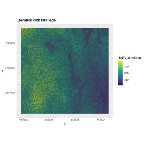
We can layer another raster on top of our hillshade by adding another
call to the geom_raster() function. Let’s overlay
DSM_HARV on top of the hill_HARV.
R
ggplot() +
  geom_raster(data = DSM_HARV_df ,
              aes(x = x, y = y,
                  fill = HARV_dsmCrop)) +
  geom_raster(data = DSM_hill_HARV_df,
              aes(x = x, y = y,
                  alpha = HARV_DSMhill)) +
  scale_fill_viridis_c() +
  scale_alpha(range = c(0.15, 0.65), guide = "none") +
  ggtitle("Elevation with hillshade") +
  coord_quickmap()
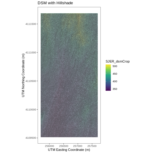
Challenge: Create DTM & DSM for SJER
Use the files in the
data/NEON-DS-Airborne-Remote-Sensing/SJER/ directory to
create a Digital Terrain Model map and Digital Surface Model map of the
San Joaquin Experimental Range field site.
Make sure to:
- include hillshade in the maps,
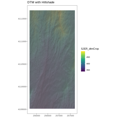
- label axes on the DSM map and exclude them from the DTM map,
- include a title for each map,
- experiment with various alpha values and color palettes to represent the data.
R
# CREATE DSM MAPS

# import DSM data
DSM_SJER <-
  rast("data/NEON-DS-Airborne-Remote-Sensing/SJER/DSM/SJER_dsmCrop.tif")
# convert to a df for plotting
DSM_SJER_df <- as.data.frame(DSM_SJER, xy = TRUE)

# import DSM hillshade
DSM_hill_SJER <-
  rast("data/NEON-DS-Airborne-Remote-Sensing/SJER/DSM/SJER_dsmHill.tif")
# convert to a df for plotting
DSM_hill_SJER_df <- as.data.frame(DSM_hill_SJER, xy = TRUE)

# Build Plot
ggplot() +
    geom_raster(data = DSM_SJER_df ,
                aes(x = x, y = y,
                     fill = SJER_dsmCrop,
                     alpha = 0.8)
                ) +
    geom_raster(data = DSM_hill_SJER_df,
                aes(x = x, y = y,
                  alpha = SJER_dsmHill)
                ) +
    scale_fill_viridis_c() +
    guides(fill = guide_colorbar()) +
    scale_alpha(range = c(0.4, 0.7), guide = "none") +
    # remove grey background and grid lines
    theme_bw() +
    theme(panel.grid.major = element_blank(),
          panel.grid.minor = element_blank()) +
    xlab("UTM Easting Coordinate (m)") +
    ylab("UTM Northing Coordinate (m)") +
    ggtitle("DSM with Hillshade") +
    coord_quickmap()
R
# CREATE DTM MAP
# import DTM
DTM_SJER <-
  rast("data/NEON-DS-Airborne-Remote-Sensing/SJER/DTM/SJER_dtmCrop.tif")
DTM_SJER_df <- as.data.frame(DTM_SJER, xy = TRUE)

# DTM Hillshade
DTM_hill_SJER <-
  rast("data/NEON-DS-Airborne-Remote-Sensing/SJER/DTM/SJER_dtmHill.tif")
DTM_hill_SJER_df <- as.data.frame(DTM_hill_SJER, xy = TRUE)

ggplot() +
    geom_raster(data = DTM_SJER_df ,
                aes(x = x, y = y,
                     fill = SJER_dtmCrop,
                     alpha = 2.0)
                ) +
    geom_raster(data = DTM_hill_SJER_df,
                aes(x = x, y = y,
                  alpha = SJER_dtmHill)
                ) +
    scale_fill_viridis_c() +
    guides(fill = guide_colorbar()) +
    scale_alpha(range = c(0.4, 0.7), guide = "none") +
    theme_bw() +
    theme(panel.grid.major = element_blank(),
          panel.grid.minor = element_blank()) +
    theme(axis.title.x = element_blank(),
          axis.title.y = element_blank()) +
    ggtitle("DTM with Hillshade") +
    coord_quickmap()
Key Points
- Continuous data ranges can be grouped into categories using
mutate()andcut(). - Use built-in
terrain.colors()or set your preferred color scheme manually. - Layer rasters on top of one another by using the
alphaaesthetic.
Content from Reproject Raster Data
Last updated on 2024-10-15 | Edit this page
Overview
Questions
- How do I work with raster data sets that are in different projections?
Objectives
- Reproject a raster in R.
Things You’ll Need To Complete This Episode
See the lesson homepage for detailed information about the software, data, and other prerequisites you will need to work through the examples in this episode.
Sometimes we encounter raster datasets that do not “line up” when
plotted or analyzed. Rasters that don’t line up are most often in
different Coordinate Reference Systems (CRS). This episode explains how
to deal with rasters in different, known CRSs. It will walk though
reprojecting rasters in R using the project() function in
the terra package.
Raster Projection in R
In the Plot Raster Data in R episode, we learned how to layer a raster file on top of a hillshade for a nice looking basemap. In that episode, all of our data were in the same CRS. What happens when things don’t line up?
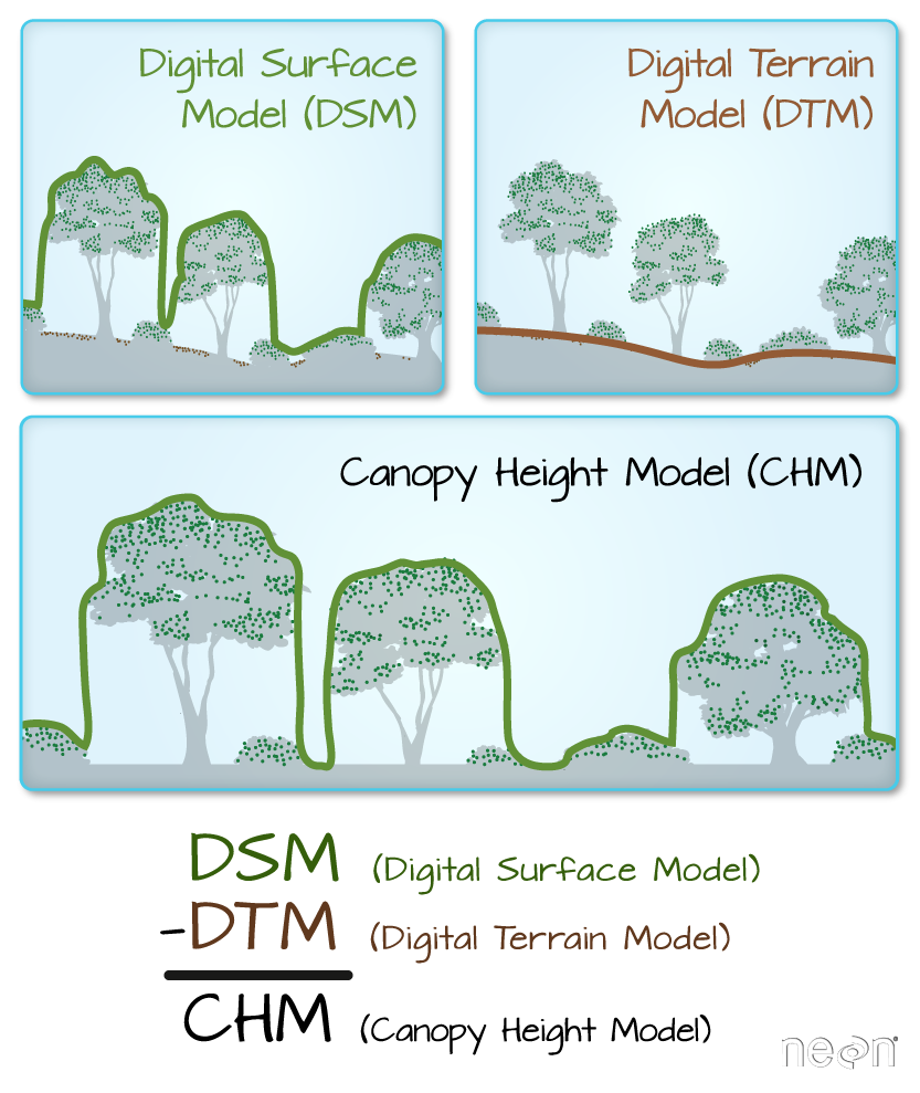
For this episode, we will be working with the Harvard Forest Digital Terrain Model data. This differs from the surface model data we’ve been working with so far in that the digital surface model (DSM) includes the tops of trees, while the digital terrain model (DTM) shows the ground level.
We’ll be looking at another model (the canopy height model) in a later episode and will see how
to calculate the CHM from the DSM and DTM. Here, we will create a map of
the Harvard Forest Digital Terrain Model (DTM_HARV) draped
or layered on top of the hillshade (DTM_hill_HARV). The
hillshade layer maps the terrain using light and shadow to create a
3D-looking image, based on a hypothetical illumination of the ground
level.
First, we need to import the DTM and DTM hillshade data.
R
DTM_HARV <-
    rast("data/NEON-DS-Airborne-Remote-Sensing/HARV/DTM/HARV_dtmCrop.tif")

DTM_hill_HARV <-
    rast("data/NEON-DS-Airborne-Remote-Sensing/HARV/DTM/HARV_DTMhill_WGS84.tif")
Next, we will convert each of these datasets to a dataframe for
plotting with ggplot.
R
DTM_HARV_df <- as.data.frame(DTM_HARV, xy = TRUE)

DTM_hill_HARV_df <- as.data.frame(DTM_hill_HARV, xy = TRUE)
Now we can create a map of the DTM layered over the hillshade.
R
ggplot() +
     geom_raster(data = DTM_HARV_df ,
                 aes(x = x, y = y,
                  fill = HARV_dtmCrop)) +
     geom_raster(data = DTM_hill_HARV_df,
                 aes(x = x, y = y,
                   alpha = HARV_DTMhill_WGS84)) +
     scale_fill_gradientn(name = "Elevation", colors = terrain.colors(10)) +
     coord_quickmap()
Our results are curious - neither the Digital Terrain Model
(DTM_HARV_df) nor the DTM Hillshade
(DTM_hill_HARV_df) plotted. Let’s try to plot the DTM on
its own to make sure there are data there.
R
ggplot() +
geom_raster(data = DTM_HARV_df,
    aes(x = x, y = y,
    fill = HARV_dtmCrop)) +
scale_fill_gradientn(name = "Elevation", colors = terrain.colors(10)) +
coord_quickmap()

Our DTM seems to contain data and plots just fine.
Next we plot the DTM Hillshade on its own to see whether everything is OK.
R
ggplot() +
geom_raster(data = DTM_hill_HARV_df,
    aes(x = x, y = y,
    alpha = HARV_DTMhill_WGS84)) +
    coord_quickmap()
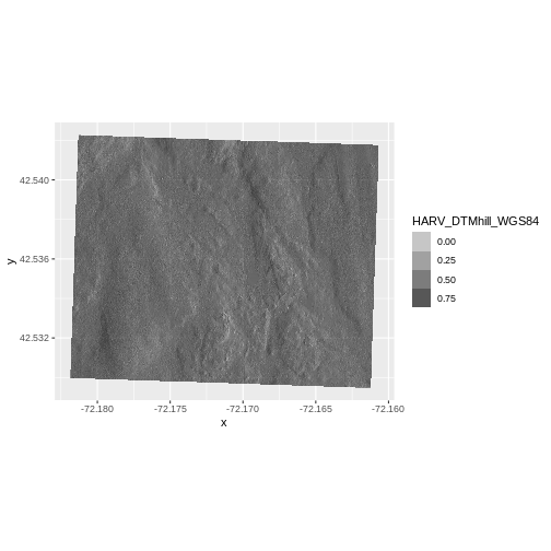
If we look at the axes, we can see that the projections of the two
rasters are different. When this is the case, ggplot won’t
render the image. It won’t even throw an error message to tell you
something has gone wrong. We can look at Coordinate Reference Systems
(CRSs) of the DTM and the hillshade data to see how they differ.
Exercise
View the CRS for each of these two datasets. What projection does each use?
R
# view crs for DTM
crs(DTM_HARV, parse = TRUE)
OUTPUT
 [1] "PROJCRS[\"WGS 84 / UTM zone 18N\","
 [2] "    BASEGEOGCRS[\"WGS 84\","
 [3] "        DATUM[\"World Geodetic System 1984\","
 [4] "            ELLIPSOID[\"WGS 84\",6378137,298.257223563,"
 [5] "                LENGTHUNIT[\"metre\",1]]],"
 [6] "        PRIMEM[\"Greenwich\",0,"
 [7] "            ANGLEUNIT[\"degree\",0.0174532925199433]],"
 [8] "        ID[\"EPSG\",4326]],"
 [9] "    CONVERSION[\"UTM zone 18N\","
[10] "        METHOD[\"Transverse Mercator\","
[11] "            ID[\"EPSG\",9807]],"
[12] "        PARAMETER[\"Latitude of natural origin\",0,"
[13] "            ANGLEUNIT[\"degree\",0.0174532925199433],"
[14] "            ID[\"EPSG\",8801]],"
[15] "        PARAMETER[\"Longitude of natural origin\",-75,"
[16] "            ANGLEUNIT[\"degree\",0.0174532925199433],"
[17] "            ID[\"EPSG\",8802]],"
[18] "        PARAMETER[\"Scale factor at natural origin\",0.9996,"
[19] "            SCALEUNIT[\"unity\",1],"
[20] "            ID[\"EPSG\",8805]],"
[21] "        PARAMETER[\"False easting\",500000,"
[22] "            LENGTHUNIT[\"metre\",1],"
[23] "            ID[\"EPSG\",8806]],"
[24] "        PARAMETER[\"False northing\",0,"
[25] "            LENGTHUNIT[\"metre\",1],"
[26] "            ID[\"EPSG\",8807]]],"
[27] "    CS[Cartesian,2],"
[28] "        AXIS[\"(E)\",east,"
[29] "            ORDER[1],"
[30] "            LENGTHUNIT[\"metre\",1]],"
[31] "        AXIS[\"(N)\",north,"
[32] "            ORDER[2],"
[33] "            LENGTHUNIT[\"metre\",1]],"
[34] "    USAGE["
[35] "        SCOPE[\"Engineering survey, topographic mapping.\"],"
[36] "        AREA[\"Between 78°W and 72°W, northern hemisphere between equator and 84°N, onshore and offshore. Bahamas. Canada - Nunavut; Ontario; Quebec. Colombia. Cuba. Ecuador. Greenland. Haiti. Jamica. Panama. Turks and Caicos Islands. United States (USA). Venezuela.\"],"
[37] "        BBOX[0,-78,84,-72]],"
[38] "    ID[\"EPSG\",32618]]"
R
# view crs for hillshade
crs(DTM_hill_HARV, parse = TRUE)
OUTPUT
 [1] "GEOGCRS[\"WGS 84\","
 [2] "    DATUM[\"World Geodetic System 1984\","
 [3] "        ELLIPSOID[\"WGS 84\",6378137,298.257223563,"
 [4] "            LENGTHUNIT[\"metre\",1]]],"
 [5] "    PRIMEM[\"Greenwich\",0,"
 [6] "        ANGLEUNIT[\"degree\",0.0174532925199433]],"
 [7] "    CS[ellipsoidal,2],"
 [8] "        AXIS[\"geodetic latitude (Lat)\",north,"
 [9] "            ORDER[1],"
[10] "            ANGLEUNIT[\"degree\",0.0174532925199433]],"
[11] "        AXIS[\"geodetic longitude (Lon)\",east,"
[12] "            ORDER[2],"
[13] "            ANGLEUNIT[\"degree\",0.0174532925199433]],"
[14] "    ID[\"EPSG\",4326]]"
DTM_HARV is in the UTM projection, with units of meters.
DTM_hill_HARV is in Geographic WGS84 - which
is represented by latitude and longitude values.
Because the two rasters are in different CRSs, they don’t line up
when plotted in R. We need to reproject (or change the projection of)
DTM_hill_HARV into the UTM CRS. Alternatively, we could
reproject DTM_HARV into WGS84.
Reproject Rasters
We can use the project() function to reproject a raster
into a new CRS. Keep in mind that reprojection only works when you first
have a defined CRS for the raster object that you want to reproject. It
cannot be used if no CRS is defined. Lucky for us, the
DTM_hill_HARV has a defined CRS.
Data Tip
When we reproject a raster, we move it from one “grid” to another. Thus, we are modifying the data! Keep this in mind as we work with raster data.
To use the project() function, we need to define two
things:
- the object we want to reproject and
- the CRS that we want to reproject it to.
The syntax is project(RasterObject, crs)
We want the CRS of our hillshade to match the DTM_HARV
raster. We can thus assign the CRS of our DTM_HARV to our
hillshade within the project() function as follows:
crs(DTM_HARV). Note that we are using the
project() function on the raster object, not the
data.frame() we use for plotting with
ggplot.
First we will reproject our DTM_hill_HARV raster data to
match the DTM_HARV raster CRS:
R
DTM_hill_UTMZ18N_HARV <- project(DTM_hill_HARV,
                                 crs(DTM_HARV))
Now we can compare the CRS of our original DTM hillshade and our new DTM hillshade, to see how they are different.
R
crs(DTM_hill_UTMZ18N_HARV, parse = TRUE)
OUTPUT
 [1] "PROJCRS[\"WGS 84 / UTM zone 18N\","
 [2] "    BASEGEOGCRS[\"WGS 84\","
 [3] "        DATUM[\"World Geodetic System 1984\","
 [4] "            ELLIPSOID[\"WGS 84\",6378137,298.257223563,"
 [5] "                LENGTHUNIT[\"metre\",1]]],"
 [6] "        PRIMEM[\"Greenwich\",0,"
 [7] "            ANGLEUNIT[\"degree\",0.0174532925199433]],"
 [8] "        ID[\"EPSG\",4326]],"
 [9] "    CONVERSION[\"UTM zone 18N\","
[10] "        METHOD[\"Transverse Mercator\","
[11] "            ID[\"EPSG\",9807]],"
[12] "        PARAMETER[\"Latitude of natural origin\",0,"
[13] "            ANGLEUNIT[\"degree\",0.0174532925199433],"
[14] "            ID[\"EPSG\",8801]],"
[15] "        PARAMETER[\"Longitude of natural origin\",-75,"
[16] "            ANGLEUNIT[\"degree\",0.0174532925199433],"
[17] "            ID[\"EPSG\",8802]],"
[18] "        PARAMETER[\"Scale factor at natural origin\",0.9996,"
[19] "            SCALEUNIT[\"unity\",1],"
[20] "            ID[\"EPSG\",8805]],"
[21] "        PARAMETER[\"False easting\",500000,"
[22] "            LENGTHUNIT[\"metre\",1],"
[23] "            ID[\"EPSG\",8806]],"
[24] "        PARAMETER[\"False northing\",0,"
[25] "            LENGTHUNIT[\"metre\",1],"
[26] "            ID[\"EPSG\",8807]]],"
[27] "    CS[Cartesian,2],"
[28] "        AXIS[\"(E)\",east,"
[29] "            ORDER[1],"
[30] "            LENGTHUNIT[\"metre\",1]],"
[31] "        AXIS[\"(N)\",north,"
[32] "            ORDER[2],"
[33] "            LENGTHUNIT[\"metre\",1]],"
[34] "    USAGE["
[35] "        SCOPE[\"Engineering survey, topographic mapping.\"],"
[36] "        AREA[\"Between 78°W and 72°W, northern hemisphere between equator and 84°N, onshore and offshore. Bahamas. Canada - Nunavut; Ontario; Quebec. Colombia. Cuba. Ecuador. Greenland. Haiti. Jamica. Panama. Turks and Caicos Islands. United States (USA). Venezuela.\"],"
[37] "        BBOX[0,-78,84,-72]],"
[38] "    ID[\"EPSG\",32618]]"
R
crs(DTM_hill_HARV, parse = TRUE)
OUTPUT
 [1] "GEOGCRS[\"WGS 84\","
 [2] "    DATUM[\"World Geodetic System 1984\","
 [3] "        ELLIPSOID[\"WGS 84\",6378137,298.257223563,"
 [4] "            LENGTHUNIT[\"metre\",1]]],"
 [5] "    PRIMEM[\"Greenwich\",0,"
 [6] "        ANGLEUNIT[\"degree\",0.0174532925199433]],"
 [7] "    CS[ellipsoidal,2],"
 [8] "        AXIS[\"geodetic latitude (Lat)\",north,"
 [9] "            ORDER[1],"
[10] "            ANGLEUNIT[\"degree\",0.0174532925199433]],"
[11] "        AXIS[\"geodetic longitude (Lon)\",east,"
[12] "            ORDER[2],"
[13] "            ANGLEUNIT[\"degree\",0.0174532925199433]],"
[14] "    ID[\"EPSG\",4326]]"
We can also compare the extent of the two objects.
R
ext(DTM_hill_UTMZ18N_HARV)
OUTPUT
SpatExtent : 731402.31567604, 733200.22199435, 4712407.19751409, 4713901.78222079 (xmin, xmax, ymin, ymax)R
ext(DTM_hill_HARV)
OUTPUT
SpatExtent : -72.1819236223343, -72.1606102223342, 42.5294079700285, 42.5423355900285 (xmin, xmax, ymin, ymax)Notice in the output above that the crs() of
DTM_hill_UTMZ18N_HARV is now UTM. However, the extent
values of DTM_hillUTMZ18N_HARV are different from
DTM_hill_HARV.
Challenge: Extent Change with CRS Change
Why do you think the two extents differ?
The extent for DTM_hill_UTMZ18N_HARV is in UTMs so the extent is in meters. The extent for DTM_hill_HARV is in lat/long so the extent is expressed in decimal degrees.
Deal with Raster Resolution
Let’s next have a look at the resolution of our reprojected hillshade versus our original data.
R
res(DTM_hill_UTMZ18N_HARV)
OUTPUT
[1] 1.001061 1.001061R
res(DTM_HARV)
OUTPUT
[1] 1 1These two resolutions are different, but they’re representing the
same data. We can tell R to force our newly reprojected raster to be 1m
x 1m resolution by adding a line of code res=1 within the
project() function. In the example below, we ensure a
resolution match by using res(DTM_HARV) as a variable.
R
  DTM_hill_UTMZ18N_HARV <- project(DTM_hill_HARV,
                                   crs(DTM_HARV),
                                   res = res(DTM_HARV))
Now both our resolutions and our CRSs match, so we can plot these two data sets together. Let’s double-check our resolution to be sure:
R
res(DTM_hill_UTMZ18N_HARV)
OUTPUT
[1] 1 1R
res(DTM_HARV)
OUTPUT
[1] 1 1For plotting with ggplot(), we will need to create a
dataframe from our newly reprojected raster.
R
DTM_hill_HARV_2_df <- as.data.frame(DTM_hill_UTMZ18N_HARV, xy = TRUE)
We can now create a plot of this data.
R
ggplot() +
     geom_raster(data = DTM_HARV_df ,
                 aes(x = x, y = y,
                  fill = HARV_dtmCrop)) +
     geom_raster(data = DTM_hill_HARV_2_df,
                 aes(x = x, y = y,
                   alpha = HARV_DTMhill_WGS84)) +
     scale_fill_gradientn(name = "Elevation", colors = terrain.colors(10)) +
     coord_quickmap()
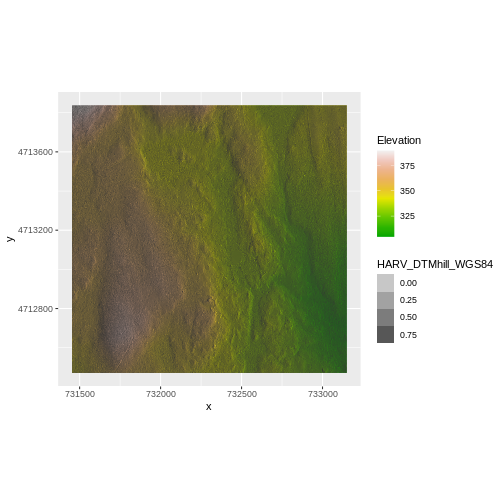
We have now successfully draped the Digital Terrain Model on top of our hillshade to produce a nice looking, textured map!
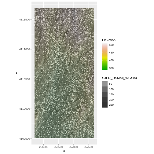
Challenge: Reproject, then Plot a Digital Terrain Model
Create a map of the San
Joaquin Experimental Range field site using the
SJER_DSMhill_WGS84.tif and SJER_dsmCrop.tif
files.
Reproject the data as necessary to make things line up!
R
# import DSM
DSM_SJER <-
    rast("data/NEON-DS-Airborne-Remote-Sensing/SJER/DSM/SJER_dsmCrop.tif")
# import DSM hillshade
DSM_hill_SJER_WGS <-
    rast("data/NEON-DS-Airborne-Remote-Sensing/SJER/DSM/SJER_DSMhill_WGS84.tif")

# reproject raster
DSM_hill_UTMZ18N_SJER <- project(DSM_hill_SJER_WGS,
                                 crs(DSM_SJER),
                                 res = 1)

# convert to data.frames
DSM_SJER_df <- as.data.frame(DSM_SJER, xy = TRUE)

DSM_hill_SJER_df <- as.data.frame(DSM_hill_UTMZ18N_SJER, xy = TRUE)

ggplot() +
     geom_raster(data = DSM_hill_SJER_df,
                 aes(x = x, y = y,
                   alpha = SJER_DSMhill_WGS84)
                 ) +
     geom_raster(data = DSM_SJER_df,
             aes(x = x, y = y,
                  fill = SJER_dsmCrop,
                  alpha=0.8)
             ) +
     scale_fill_gradientn(name = "Elevation", colors = terrain.colors(10)) +
     coord_quickmap()
Challenge: Reproject, then Plot a Digital Terrain Model (continued)
If you completed the San Joaquin plotting challenge in the Plot Raster Data in R episode, how does the map you just created compare to that map?
The maps look identical. Which is what they should be as the only difference is this one was reprojected from WGS84 to UTM prior to plotting.
Key Points
- In order to plot two raster data sets together, they must be in the same CRS.
- Use the
project()function to convert between CRSs.
Content from Raster Calculations
Last updated on 2024-10-15 | Edit this page
Overview
Questions
- How do I subtract one raster from another and extract pixel values for defined locations?
Objectives
- Perform a subtraction between two rasters using raster math.
- Perform a more efficient subtraction between two rasters using the
raster
lapp()function. - Export raster data as a GeoTIFF file.
Things You’ll Need To Complete This Episode
See the lesson homepage for detailed information about the software, data, and other prerequisites you will need to work through the examples in this episode.
We often want to combine values of and perform calculations on
rasters to create a new output raster. This episode covers how to
subtract one raster from another using basic raster math and the
lapp() function. It also covers how to extract pixel values
from a set of locations - for example a buffer region around plot
locations at a field site.
Raster Calculations in R
We often want to perform calculations on two or more rasters to create a new output raster. For example, if we are interested in mapping the heights of trees across an entire field site, we might want to calculate the difference between the Digital Surface Model (DSM, tops of trees) and the Digital Terrain Model (DTM, ground level). The resulting dataset is referred to as a Canopy Height Model (CHM) and represents the actual height of trees, buildings, etc. with the influence of ground elevation removed.
More Resources
- Check out more on LiDAR CHM, DTM and DSM in this NEON Data Skills overview tutorial: What is a CHM, DSM and DTM? About Gridded, Raster LiDAR Data.
Load the Data
For this episode, we will use the DTM and DSM from the NEON Harvard Forest Field site and San Joaquin Experimental Range, which we already have loaded from previous episodes.
Exercise
Use the describe() function to view information about
the DTM and DSM data files. Do the two rasters have the same or
different CRSs and resolutions? Do they both have defined minimum and
maximum values?
R
describe("data/NEON-DS-Airborne-Remote-Sensing/HARV/DTM/HARV_dtmCrop.tif")
OUTPUT
 [1] "Driver: GTiff/GeoTIFF"
 [2] "Files: data/NEON-DS-Airborne-Remote-Sensing/HARV/DTM/HARV_dtmCrop.tif"
 [3] "Size is 1697, 1367"
 [4] "Coordinate System is:"
 [5] "PROJCRS[\"WGS 84 / UTM zone 18N\","
 [6] "    BASEGEOGCRS[\"WGS 84\","
 [7] "        DATUM[\"World Geodetic System 1984\","
 [8] "            ELLIPSOID[\"WGS 84\",6378137,298.257223563,"
 [9] "                LENGTHUNIT[\"metre\",1]]],"
[10] "        PRIMEM[\"Greenwich\",0,"
[11] "            ANGLEUNIT[\"degree\",0.0174532925199433]],"
[12] "        ID[\"EPSG\",4326]],"
[13] "    CONVERSION[\"UTM zone 18N\","
[14] "        METHOD[\"Transverse Mercator\","
[15] "            ID[\"EPSG\",9807]],"
[16] "        PARAMETER[\"Latitude of natural origin\",0,"
[17] "            ANGLEUNIT[\"degree\",0.0174532925199433],"
[18] "            ID[\"EPSG\",8801]],"
[19] "        PARAMETER[\"Longitude of natural origin\",-75,"
[20] "            ANGLEUNIT[\"degree\",0.0174532925199433],"
[21] "            ID[\"EPSG\",8802]],"
[22] "        PARAMETER[\"Scale factor at natural origin\",0.9996,"
[23] "            SCALEUNIT[\"unity\",1],"
[24] "            ID[\"EPSG\",8805]],"
[25] "        PARAMETER[\"False easting\",500000,"
[26] "            LENGTHUNIT[\"metre\",1],"
[27] "            ID[\"EPSG\",8806]],"
[28] "        PARAMETER[\"False northing\",0,"
[29] "            LENGTHUNIT[\"metre\",1],"
[30] "            ID[\"EPSG\",8807]]],"
[31] "    CS[Cartesian,2],"
[32] "        AXIS[\"(E)\",east,"
[33] "            ORDER[1],"
[34] "            LENGTHUNIT[\"metre\",1]],"
[35] "        AXIS[\"(N)\",north,"
[36] "            ORDER[2],"
[37] "            LENGTHUNIT[\"metre\",1]],"
[38] "    USAGE["
[39] "        SCOPE[\"Engineering survey, topographic mapping.\"],"
[40] "        AREA[\"Between 78°W and 72°W, northern hemisphere between equator and 84°N, onshore and offshore. Bahamas. Canada - Nunavut; Ontario; Quebec. Colombia. Cuba. Ecuador. Greenland. Haiti. Jamica. Panama. Turks and Caicos Islands. United States (USA). Venezuela.\"],"
[41] "        BBOX[0,-78,84,-72]],"
[42] "    ID[\"EPSG\",32618]]"
[43] "Data axis to CRS axis mapping: 1,2"
[44] "Origin = (731453.000000000000000,4713838.000000000000000)"
[45] "Pixel Size = (1.000000000000000,-1.000000000000000)"
[46] "Metadata:"
[47] "  AREA_OR_POINT=Area"
[48] "Image Structure Metadata:"
[49] "  COMPRESSION=LZW"
[50] "  INTERLEAVE=BAND"
[51] "Corner Coordinates:"
[52] "Upper Left  (  731453.000, 4713838.000) ( 72d10'52.71\"W, 42d32'32.18\"N)"
[53] "Lower Left  (  731453.000, 4712471.000) ( 72d10'54.71\"W, 42d31'47.92\"N)"
[54] "Upper Right (  733150.000, 4713838.000) ( 72d 9'38.40\"W, 42d32'30.35\"N)"
[55] "Lower Right (  733150.000, 4712471.000) ( 72d 9'40.41\"W, 42d31'46.08\"N)"
[56] "Center      (  732301.500, 4713154.500) ( 72d10'16.56\"W, 42d32' 9.13\"N)"
[57] "Band 1 Block=1697x1 Type=Float64, ColorInterp=Gray"
[58] "  Min=304.560 Max=389.820 "
[59] "  Minimum=304.560, Maximum=389.820, Mean=344.898, StdDev=15.861"
[60] "  NoData Value=-9999"
[61] "  Metadata:"
[62] "    STATISTICS_MAXIMUM=389.81997680664"
[63] "    STATISTICS_MEAN=344.8979433625"
[64] "    STATISTICS_MINIMUM=304.55999755859"
[65] "    STATISTICS_STDDEV=15.861471000978"
R
describe("data/NEON-DS-Airborne-Remote-Sensing/HARV/DSM/HARV_dsmCrop.tif")
OUTPUT
[1] "Driver: GTiff/GeoTIFF"
[2] "Files: data/NEON-DS-Airborne-Remote-Sensing/HARV/DSM/HARV_dsmCrop.tif"
[3] "Size is 1697, 1367"
[4] "Coordinate System is:"
[5] "PROJCRS[\"WGS 84 / UTM zone 18N\","
[6] " BASEGEOGCRS[\"WGS 84\","
[7] " DATUM[\"World Geodetic System 1984\","
[8] " ELLIPSOID[\"WGS 84\",6378137,298.257223563,"
[9] " LENGTHUNIT[\"metre\",1]]],"
[10] " PRIMEM[\"Greenwich\",0,"
[11] " ANGLEUNIT[\"degree\",0.0174532925199433]],"
[12] " ID[\"EPSG\",4326]],"
[13] " CONVERSION[\"UTM zone 18N\","
[14] " METHOD[\"Transverse Mercator\","
[15] " ID[\"EPSG\",9807]],"
[16] " PARAMETER[\"Latitude of natural origin\",0,"
[17] " ANGLEUNIT[\"degree\",0.0174532925199433],"
[18] " ID[\"EPSG\",8801]],"
[19] " PARAMETER[\"Longitude of natural origin\",-75,"
[20] " ANGLEUNIT[\"degree\",0.0174532925199433],"
[21] " ID[\"EPSG\",8802]],"
[22] " PARAMETER[\"Scale factor at natural origin\",0.9996,"
[23] " SCALEUNIT[\"unity\",1],"
[24] " ID[\"EPSG\",8805]],"
[25] " PARAMETER[\"False easting\",500000,"
[26] " LENGTHUNIT[\"metre\",1],"
[27] " ID[\"EPSG\",8806]],"
[28] " PARAMETER[\"False northing\",0,"
[29] " LENGTHUNIT[\"metre\",1],"
[30] " ID[\"EPSG\",8807]]],"
[31] " CS[Cartesian,2],"
[32] " AXIS[\"(E)\",east,"
[33] " ORDER[1],"
[34] " LENGTHUNIT[\"metre\",1]],"
[35] " AXIS[\"(N)\",north,"
[36] " ORDER[2],"
[37] " LENGTHUNIT[\"metre\",1]],"
[38] " USAGE["
[39] " SCOPE[\"Engineering survey, topographic mapping.\"],"
[40] " AREA[\"Between 78°W and 72°W, northern hemisphere between equator and 84°N, onshore and offshore. Bahamas. Canada - Nunavut; Ontario; Quebec. Colombia. Cuba. Ecuador. Greenland. Haiti. Jamica. Panama. Turks and Caicos Islands. United States (USA). Venezuela.\"],"
[41] " BBOX[0,-78,84,-72]],"
[42] " ID[\"EPSG\",32618]]"
[43] "Data axis to CRS axis mapping: 1,2"
[44] "Origin = (731453.000000000000000,4713838.000000000000000)"
[45] "Pixel Size = (1.000000000000000,-1.000000000000000)"
[46] "Metadata:"
[47] " AREA_OR_POINT=Area"
[48] "Image Structure Metadata:"
[49] " COMPRESSION=LZW"
[50] " INTERLEAVE=BAND"
[51] "Corner Coordinates:"
[52] "Upper Left ( 731453.000, 4713838.000) ( 72d10'52.71\"W, 42d32'32.18\"N)"
[53] "Lower Left ( 731453.000, 4712471.000) ( 72d10'54.71\"W, 42d31'47.92\"N)"
[54] "Upper Right ( 733150.000, 4713838.000) ( 72d 9'38.40\"W, 42d32'30.35\"N)"
[55] "Lower Right ( 733150.000, 4712471.000) ( 72d 9'40.41\"W, 42d31'46.08\"N)"
[56] "Center ( 732301.500, 4713154.500) ( 72d10'16.56\"W, 42d32' 9.13\"N)"
[57] "Band 1 Block=1697x1 Type=Float64, ColorInterp=Gray"
[58] " Min=305.070 Max=416.070 "
[59] " Minimum=305.070, Maximum=416.070, Mean=359.853, StdDev=17.832"
[60] " NoData Value=-9999"
[61] " Metadata:"
[62] " STATISTICS_MAXIMUM=416.06997680664"
[63] " STATISTICS_MEAN=359.85311802914"
[64] " STATISTICS_MINIMUM=305.07000732422"
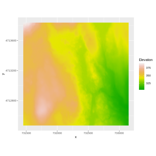
[65] " STATISTICS_STDDEV=17.83169335933" We’ve already loaded and worked with these two data files in earlier episodes. Let’s plot them each once more to remind ourselves what this data looks like. First we’ll plot the DTM elevation data:
R
 ggplot() +
      geom_raster(data = DTM_HARV_df ,
              aes(x = x, y = y, fill = HARV_dtmCrop)) +
     scale_fill_gradientn(name = "Elevation", colors = terrain.colors(10)) +
     coord_quickmap()
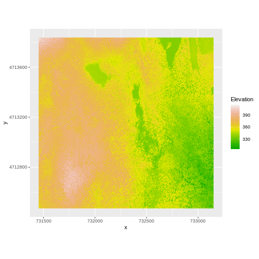
And then the DSM elevation data:
R
 ggplot() +
      geom_raster(data = DSM_HARV_df ,
              aes(x = x, y = y, fill = HARV_dsmCrop)) +
     scale_fill_gradientn(name = "Elevation", colors = terrain.colors(10)) +
     coord_quickmap()
Two Ways to Perform Raster Calculations
We can calculate the difference between two rasters in two different ways:
- by directly subtracting the two rasters in R using raster math
or for more efficient processing - particularly if our rasters are large and/or the calculations we are performing are complex:
- using the
lapp()function.
Raster Math & Canopy Height Models
We can perform raster calculations by subtracting (or adding, multiplying, etc) two rasters. In the geospatial world, we call this “raster math”.
Let’s subtract the DTM from the DSM to create a Canopy Height Model.
After subtracting, let’s create a dataframe so we can plot with
ggplot.
R
CHM_HARV <- DSM_HARV - DTM_HARV

CHM_HARV_df <- as.data.frame(CHM_HARV, xy = TRUE)
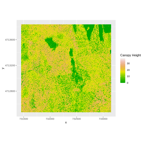
We can now plot the output CHM.
R
 ggplot() +
   geom_raster(data = CHM_HARV_df ,
               aes(x = x, y = y, fill = HARV_dsmCrop)) +
   scale_fill_gradientn(name = "Canopy Height", colors = terrain.colors(10)) +
   coord_quickmap()
Let’s have a look at the distribution of values in our newly created Canopy Height Model (CHM).
R
ggplot(CHM_HARV_df) +
    geom_histogram(aes(HARV_dsmCrop))
OUTPUT
`stat_bin()` using `bins = 30`. Pick better value with `binwidth`.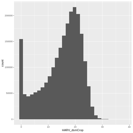
Notice that the range of values for the output CHM is between 0 and 30 meters. Does this make sense for trees in Harvard Forest?
Challenge: Explore CHM Raster Values
It’s often a good idea to explore the range of values in a raster dataset just like we might explore a dataset that we collected in the field.
- What is the min and maximum value for the Harvard Forest Canopy
Height Model (
CHM_HARV) that we just created? - What are two ways you can check this range of data for
CHM_HARV? - What is the distribution of all the pixel values in the CHM?
- Plot a histogram with 6 bins instead of the default and change the color of the histogram.
- Plot the
CHM_HARVraster using breaks that make sense for the data. Include an appropriate color palette for the data, plot title and no axes ticks / labels.
- There are missing values in our data, so we need to specify
na.rm = TRUE.
R
min(CHM_HARV_df$HARV_dsmCrop, na.rm = TRUE)
OUTPUT
[1] 0R
max(CHM_HARV_df$HARV_dsmCrop, na.rm = TRUE)
OUTPUT
[1] 38.16998- Possible ways include:
- Create a histogram
- Use the
min(),max(), andrange()functions. - Print the object and look at the
valuesattribute.
R
ggplot(CHM_HARV_df) +
    geom_histogram(aes(HARV_dsmCrop))
OUTPUT
`stat_bin()` using `bins = 30`. Pick better value with `binwidth`.
R
ggplot(CHM_HARV_df) +
    geom_histogram(aes(HARV_dsmCrop), colour="black",
                   fill="darkgreen", bins = 6)
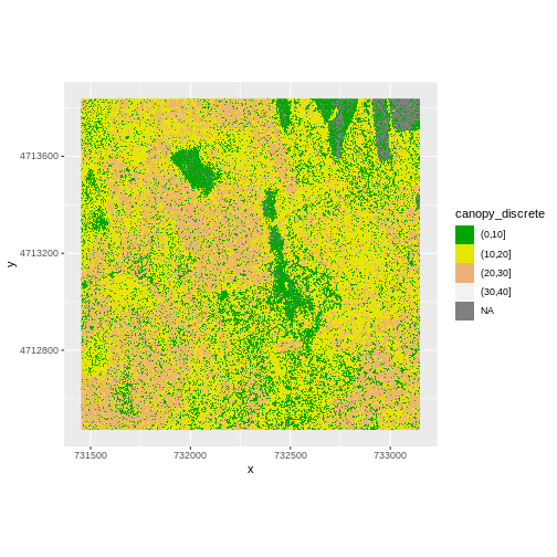
R
custom_bins <- c(0, 10, 20, 30, 40)
CHM_HARV_df <- CHM_HARV_df %>%
                  mutate(canopy_discrete = cut(HARV_dsmCrop,
                                               breaks = custom_bins))

ggplot() +
  geom_raster(data = CHM_HARV_df , aes(x = x, y = y,
                                       fill = canopy_discrete)) +
     scale_fill_manual(values = terrain.colors(4)) +
     coord_quickmap()
Efficient Raster Calculations
Raster math, like we just did, is an appropriate approach to raster calculations if:
- The rasters we are using are small in size.
- The calculations we are performing are simple.
However, raster math is a less efficient approach as computation becomes more complex or as file sizes become large.
The lapp() function takes two or more rasters and
applies a function to them using efficient processing methods. The
syntax is
outputRaster <- lapp(x, fun=functionName)
In which raster can be either a SpatRaster or a SpatRasterDataset
which is an object that holds rasters. See help(sds).
Data Tip
To create a SpatRasterDataset, we call the function sds
which can take a list of raster objects (each one created by calling
rast).
Let’s perform the same subtraction calculation that we calculated
above using raster math, using the lapp() function.
Data Tip
A custom function consists of a defined set of commands performed on
a input object. Custom functions are particularly useful for tasks that
need to be repeated over and over in the code. A simplified syntax for
writing a custom function in R is:
function_name <- function(variable1, variable2) { WhatYouWantDone, WhatToReturn}
R
CHM_ov_HARV <- lapp(sds(list(DSM_HARV, DTM_HARV)),
                    fun = function(r1, r2) { return( r1 - r2) })
Next we need to convert our new object to a data frame for plotting
with ggplot.
R
CHM_ov_HARV_df <- as.data.frame(CHM_ov_HARV, xy = TRUE)
Now we can plot the CHM:
R
 ggplot() +
   geom_raster(data = CHM_ov_HARV_df,
               aes(x = x, y = y, fill = HARV_dsmCrop)) +
   scale_fill_gradientn(name = "Canopy Height", colors = terrain.colors(10)) +
   coord_quickmap()

How do the plots of the CHM created with manual raster math and the
lapp() function compare?
Export a GeoTIFF
Now that we’ve created a new raster, let’s export the data as a
GeoTIFF file using the writeRaster() function.
When we write this raster object to a GeoTIFF file we’ll name it
CHM_HARV.tiff. This name allows us to quickly remember both
what the data contains (CHM data) and for where (HARVard Forest). The
writeRaster() function by default writes the output file to
your working directory unless you specify a full file path.
We will specify the output format (“GTiff”), the no data value
NAflag = -9999. We will also tell R to overwrite any data
that is already in a file of the same name.
R
writeRaster(CHM_ov_HARV, "CHM_HARV.tiff",
            filetype="GTiff",
            overwrite=TRUE,
            NAflag=-9999)
writeRaster() Options
The function arguments that we used above include:
-
filetype: specify that the format will be
GTiffor GeoTIFF. - overwrite: If TRUE, R will overwrite any existing file with the same name in the specified directory. USE THIS SETTING WITH CAUTION!
-
NAflag: set the GeoTIFF tag for
NoDataValueto -9999, the National Ecological Observatory Network’s (NEON) standardNoDataValue.
Challenge: Explore the NEON San Joaquin Experimental Range Field Site
Data are often more interesting and powerful when we compare them across various locations. Let’s compare some data collected over Harvard Forest to data collected in Southern California. The NEON San Joaquin Experimental Range (SJER) field site located in Southern California has a very different ecosystem and climate than the NEON Harvard Forest Field Site in Massachusetts.
Import the SJER DSM and DTM raster files and create a Canopy Height
Model. Then compare the two sites. Be sure to name your R objects and
outputs carefully, as follows: objectType_SJER
(e.g. DSM_SJER). This will help you keep track of data from
different sites!
- You should have the DSM and DTM data for the SJER site already loaded from the Plot Raster Data in R episode.) Don’t forget to check the CRSs and units of the data.
- Create a CHM from the two raster layers and check to make sure the data are what you expect.
- Plot the CHM from SJER.
- Export the SJER CHM as a GeoTIFF.
- Compare the vegetation structure of the Harvard Forest and San Joaquin Experimental Range.
- Use the
lapp()function to subtract the two rasters & create the CHM.
R
CHM_ov_SJER <- lapp(sds(list(DSM_SJER, DTM_SJER)),
                       fun = function(r1, r2){ return(r1 - r2) })
Convert the output to a dataframe:
R
CHM_ov_SJER_df <- as.data.frame(CHM_ov_SJER, xy = TRUE)
Create a histogram to check that the data distribution makes sense:
R
ggplot(CHM_ov_SJER_df) +
    geom_histogram(aes(SJER_dsmCrop))
OUTPUT
`stat_bin()` using `bins = 30`. Pick better value with `binwidth`.
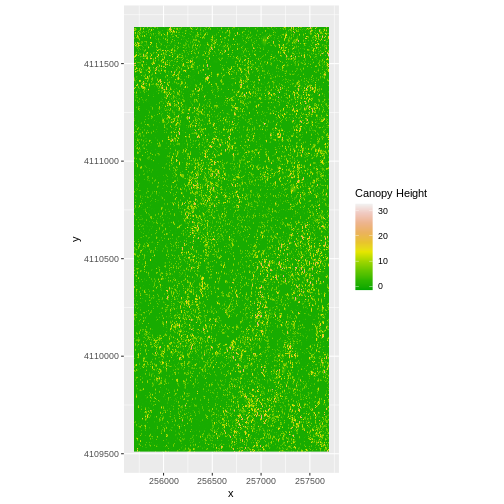
- Create a plot of the CHM:
R
 ggplot() +
      geom_raster(data = CHM_ov_SJER_df,
              aes(x = x, y = y,
                   fill = SJER_dsmCrop)
              ) +
     scale_fill_gradientn(name = "Canopy Height",
        colors = terrain.colors(10)) +
     coord_quickmap()
- Export the CHM object to a file:
R
writeRaster(CHM_ov_SJER, "chm_ov_SJER.tiff",
            filetype = "GTiff",
            overwrite = TRUE,
            NAflag = -9999)
- Compare the SJER and HARV CHMs. Tree heights are much shorter in SJER. You can confirm this by looking at the histograms of the two CHMs.
R
ggplot(CHM_HARV_df) +
    geom_histogram(aes(HARV_dsmCrop))
OUTPUT
`stat_bin()` using `bins = 30`. Pick better value with `binwidth`.
R
ggplot(CHM_ov_SJER_df) +
    geom_histogram(aes(SJER_dsmCrop))
OUTPUT
`stat_bin()` using `bins = 30`. Pick better value with `binwidth`.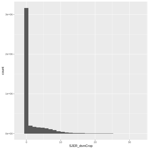
Key Points
- Rasters can be computed on using mathematical functions.
- The
lapp()function provides an efficient way to do raster math. - The
writeRaster()function can be used to write raster data to a file.
Content from Work with Multi-Band Rasters
Last updated on 2024-10-15 | Edit this page
Overview
Questions
- How can I visualize individual and multiple bands in a raster object?
Objectives
- Identify a single vs. a multi-band raster file.
- Import multi-band rasters into R using the
terrapackage. - Plot multi-band color image rasters in R using the
ggplotpackage.
Things You’ll Need To Complete This Episode
See the lesson homepage for detailed information about the software, data, and other prerequisites you will need to work through the examples in this episode.
We introduced multi-band raster data in an earlier lesson. This episode explores how to import and plot a multi-band raster in R.
Getting Started with Multi-Band Data in R
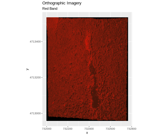
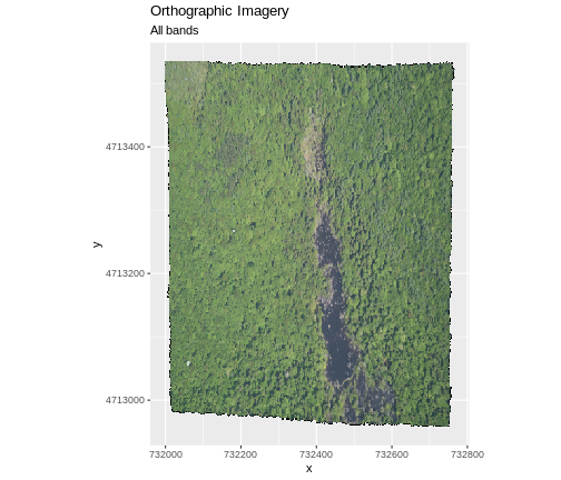
In this episode, the multi-band data that we are working with is imagery collected using the NEON Airborne Observation Platform high resolution camera over the NEON Harvard Forest field site. Each RGB image is a 3-band raster. The same steps would apply to working with a multi-spectral image with 4 or more bands - like Landsat imagery.
By using the rast() function along with the
lyrs parameter, we can read specific raster bands (i.e. the
first one); omitting this parameter would read instead all bands.
R
RGB_band1_HARV <-
  rast("data/NEON-DS-Airborne-Remote-Sensing/HARV/RGB_Imagery/HARV_RGB_Ortho.tif",
       lyrs = 1)
We need to convert this data to a data frame in order to plot it with
ggplot.
R
RGB_band1_HARV_df <- as.data.frame(RGB_band1_HARV, xy = TRUE)
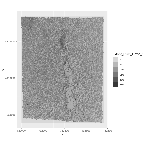
R
ggplot() +
  geom_raster(data = RGB_band1_HARV_df,
              aes(x = x, y = y, alpha = HARV_RGB_Ortho_1)) +
  coord_quickmap()
Challenge
View the attributes of this band. What are its dimensions, CRS, resolution, min and max values, and band number?
R
RGB_band1_HARV
OUTPUT
class       : SpatRaster
dimensions  : 2317, 3073, 1  (nrow, ncol, nlyr)
resolution  : 0.25, 0.25  (x, y)
extent      : 731998.5, 732766.8, 4712956, 4713536  (xmin, xmax, ymin, ymax)
coord. ref. : WGS 84 / UTM zone 18N (EPSG:32618)
source      : HARV_RGB_Ortho.tif
name        : HARV_RGB_Ortho_1
min value   :                0
max value   :              255
Notice that when we look at the attributes of this band, we see:
dimensions : 2317, 3073, 1 (nrow, ncol, nlyr)
This is R telling us that we read only one its bands.
Data Tip
The number of bands associated with a raster’s file can also be
determined using the describe() function: syntax is
describe(sources(RGB_band1_HARV)).
Image Raster Data Values
As we saw in the previous exercise, this raster contains values between 0 and 255. These values represent degrees of brightness associated with the image band. In the case of a RGB image (red, green and blue), band 1 is the red band. When we plot the red band, larger numbers (towards 255) represent pixels with more red in them (a strong red reflection). Smaller numbers (towards 0) represent pixels with less red in them (less red was reflected). To plot an RGB image, we mix red + green + blue values into one single color to create a full color image - similar to the color image a digital camera creates.
Import A Specific Band
We can use the rast() function to import specific bands
in our raster object by specifying which band we want with
lyrs = N (N represents the band number we want to work
with). To import the green band, we would use lyrs = 2.
R
RGB_band2_HARV <-
  rast("data/NEON-DS-Airborne-Remote-Sensing/HARV/RGB_Imagery/HARV_RGB_Ortho.tif",
       lyrs = 2)
We can convert this data to a data frame and plot the same way we plotted the red band:
R
RGB_band2_HARV_df <- as.data.frame(RGB_band2_HARV, xy = TRUE)
R
ggplot() +
  geom_raster(data = RGB_band2_HARV_df,
              aes(x = x, y = y, alpha = HARV_RGB_Ortho_2)) +
  coord_equal()
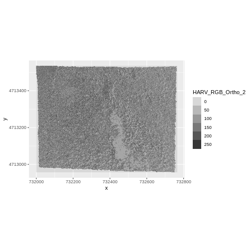
Challenge: Making Sense of Single Band Images
Compare the plots of band 1 (red) and band 2 (green). Is the forested area darker or lighter in band 2 (the green band) compared to band 1 (the red band)?
We’d expect a brighter value for the forest in band 2 (green) than in band 1 (red) because the leaves on trees of most often appear “green” - healthy leaves reflect MORE green light than red light.
Raster Stacks in R
Next, we will work with all three image bands (red, green and blue) as an R raster object. We will then plot a 3-band composite, or full color, image.
To bring in all bands of a multi-band raster, we use
therast() function.
R
RGB_stack_HARV <-
  rast("data/NEON-DS-Airborne-Remote-Sensing/HARV/RGB_Imagery/HARV_RGB_Ortho.tif")
Let’s preview the attributes of our stack object:
R
RGB_stack_HARV
OUTPUT
class       : SpatRaster
dimensions  : 2317, 3073, 3  (nrow, ncol, nlyr)
resolution  : 0.25, 0.25  (x, y)
extent      : 731998.5, 732766.8, 4712956, 4713536  (xmin, xmax, ymin, ymax)
coord. ref. : WGS 84 / UTM zone 18N (EPSG:32618)
source      : HARV_RGB_Ortho.tif
names       : HARV_RGB_Ortho_1, HARV_RGB_Ortho_2, HARV_RGB_Ortho_3
min values  :                0,                0,                0
max values  :              255,              255,              255
We can view the attributes of each band in the stack in a single output. For example, if we had hundreds of bands, we could specify which band we’d like to view attributes for using an index value:
R
RGB_stack_HARV[[2]]
OUTPUT
class       : SpatRaster
dimensions  : 2317, 3073, 1  (nrow, ncol, nlyr)
resolution  : 0.25, 0.25  (x, y)
extent      : 731998.5, 732766.8, 4712956, 4713536  (xmin, xmax, ymin, ymax)
coord. ref. : WGS 84 / UTM zone 18N (EPSG:32618)
source      : HARV_RGB_Ortho.tif
name        : HARV_RGB_Ortho_2
min value   :                0
max value   :              255
We can also use the ggplot functions to plot the data in
any layer of our raster object. Remember, we need to convert to a data
frame first.
R
RGB_stack_HARV_df <- as.data.frame(RGB_stack_HARV, xy = TRUE)
Each band in our RasterStack gets its own column in the data frame. Thus we have:
R
str(RGB_stack_HARV_df)
OUTPUT
'data.frame':	7120141 obs. of  5 variables:
 $ x               : num  731999 731999 731999 731999 732000 ...
 $ y               : num  4713535 4713535 4713535 4713535 4713535 ...
 $ HARV_RGB_Ortho_1: num  0 2 6 0 16 0 0 6 1 5 ...
 $ HARV_RGB_Ortho_2: num  1 0 9 0 5 0 4 2 1 0 ...
 $ HARV_RGB_Ortho_3: num  0 10 1 0 17 0 4 0 0 7 ...
Let’s create a histogram of the first band:
R
ggplot() +
  geom_histogram(data = RGB_stack_HARV_df, aes(HARV_RGB_Ortho_1))
OUTPUT
`stat_bin()` using `bins = 30`. Pick better value with `binwidth`.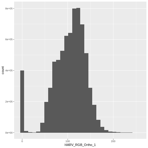
And a raster plot of the second band:
R
ggplot() +
  geom_raster(data = RGB_stack_HARV_df,
              aes(x = x, y = y, alpha = HARV_RGB_Ortho_2)) +
  coord_quickmap()
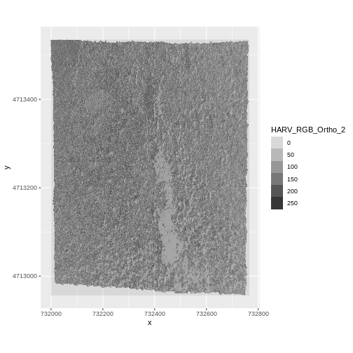
We can access any individual band in the same way.
Create A Three Band Image
To render a final three band, colored image in R, we use the
plotRGB() function.
This function allows us to:
- Identify what bands we want to render in the red, green and blue
regions. The
plotRGB()function defaults to a 1=red, 2=green, and 3=blue band order. However, you can define what bands you’d like to plot manually. Manual definition of bands is useful if you have, for example a near-infrared band and want to create a color infrared image. - Adjust the
stretchof the image to increase or decrease contrast.
Let’s plot our 3-band image. Note that we can use the
plotRGB() function directly with our RasterStack object (we
don’t need a dataframe as this function isn’t part of the
ggplot2 package).
R
plotRGB(RGB_stack_HARV,
        r = 1, g = 2, b = 3)
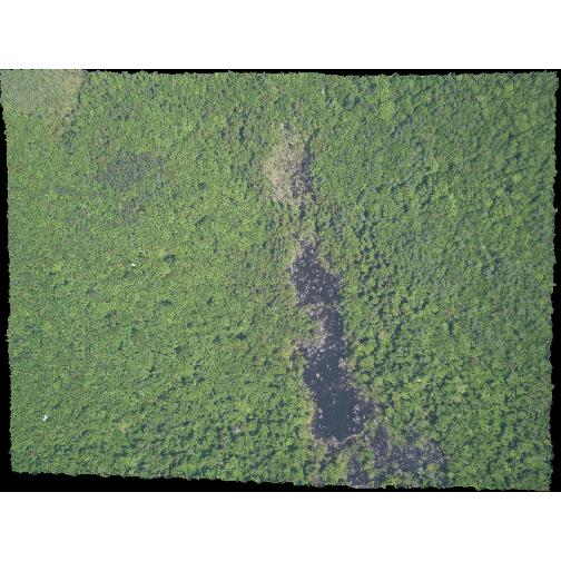
The image above looks pretty good. We can explore whether applying a
stretch to the image might improve clarity and contrast using
stretch="lin" or stretch="hist".
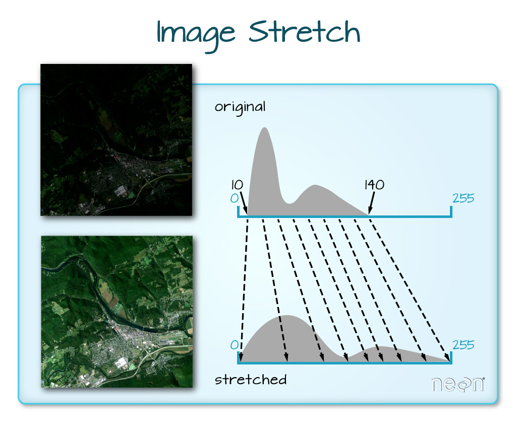
When the range of pixel brightness values is closer to 0, a darker image is rendered by default. We can stretch the values to extend to the full 0-255 range of potential values to increase the visual contrast of the image.
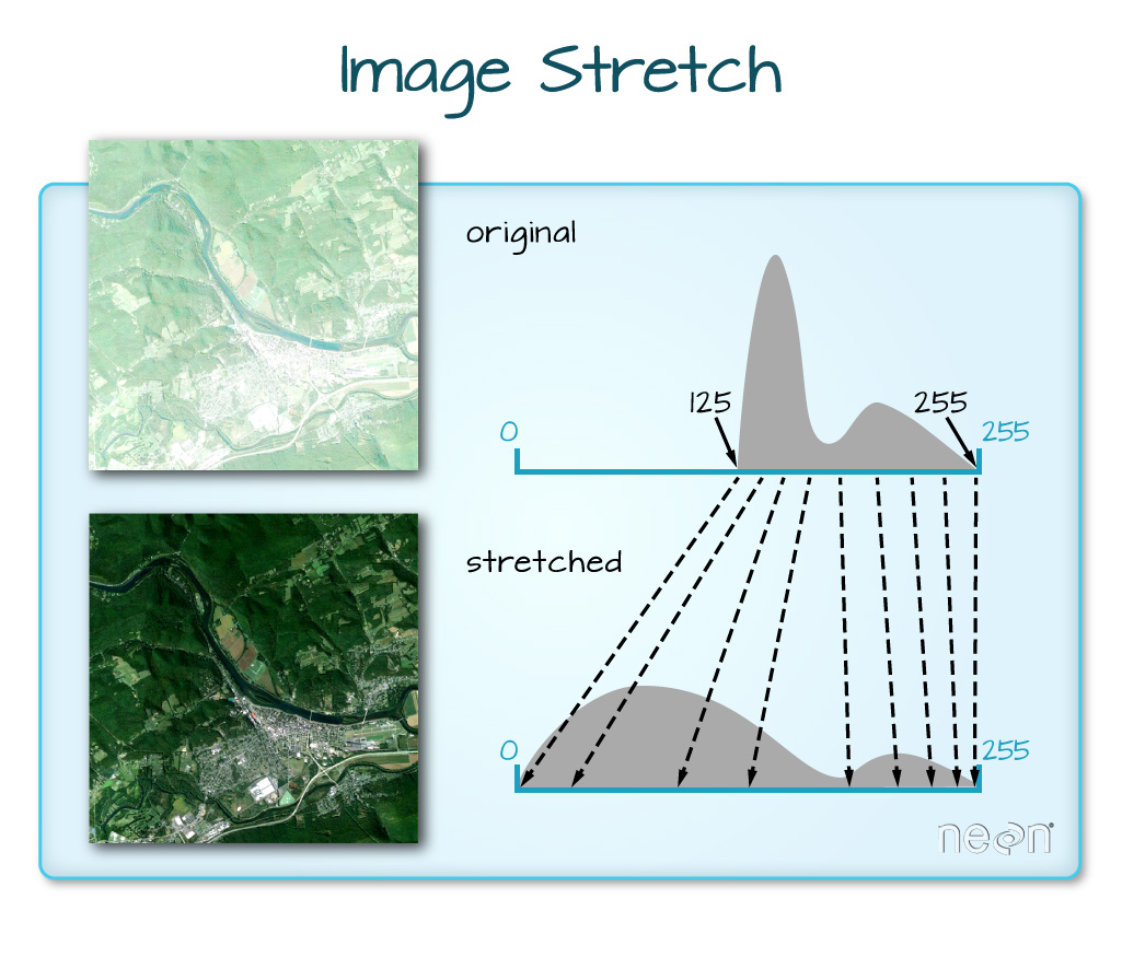
When the range of pixel brightness values is closer to 255, a lighter image is rendered by default. We can stretch the values to extend to the full 0-255 range of potential values to increase the visual contrast of the image.
R
plotRGB(RGB_stack_HARV,
        r = 1, g = 2, b = 3,
        scale = 800,
        stretch = "lin")
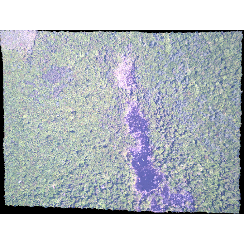
R
plotRGB(RGB_stack_HARV,
        r = 1, g = 2, b = 3,
        scale = 800,
        stretch = "hist")
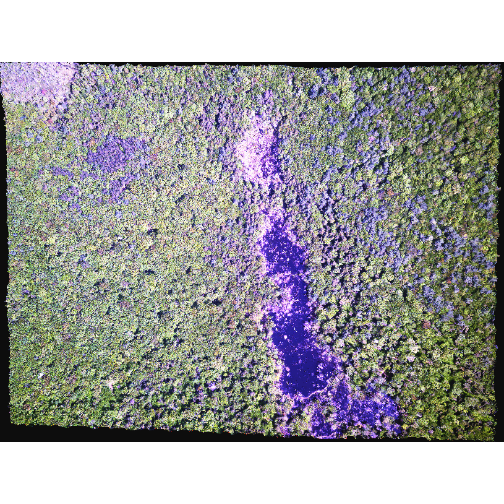
In this case, the stretch doesn’t enhance the contrast our image significantly given the distribution of reflectance (or brightness) values is distributed well between 0 and 255.
Challenge - NoData Values
Let’s explore what happens with NoData values when working with
RasterStack objects and using the plotRGB() function. We
will use the HARV_Ortho_wNA.tif GeoTIFF file in the
NEON-DS-Airborne-Remote-Sensing/HARV/RGB_Imagery/
directory.
- View the files attributes. Are there
NoDatavalues assigned for this file? - If so, what is the
NoDataValue? - How many bands does it have?
- Load the multi-band raster file into R.
- Plot the object as a true color image.
- What happened to the black edges in the data?
- What does this tell us about the difference in the data structure
between
HARV_Ortho_wNA.tifandHARV_RGB_Ortho.tif(R objectRGB_stack). How can you check?
- First we use the
describe()function to view the data attributes.
R
describe("data/NEON-DS-Airborne-Remote-Sensing/HARV/RGB_Imagery/HARV_Ortho_wNA.tif")
OUTPUT
 [1] "Driver: GTiff/GeoTIFF"
 [2] "Files: data/NEON-DS-Airborne-Remote-Sensing/HARV/RGB_Imagery/HARV_Ortho_wNA.tif"
 [3] "Size is 3073, 2317"
 [4] "Coordinate System is:"
 [5] "PROJCRS[\"WGS 84 / UTM zone 18N\","
 [6] "    BASEGEOGCRS[\"WGS 84\","
 [7] "        DATUM[\"World Geodetic System 1984\","
 [8] "            ELLIPSOID[\"WGS 84\",6378137,298.257223563,"
 [9] "                LENGTHUNIT[\"metre\",1]]],"
[10] "        PRIMEM[\"Greenwich\",0,"
[11] "            ANGLEUNIT[\"degree\",0.0174532925199433]],"
[12] "        ID[\"EPSG\",4326]],"
[13] "    CONVERSION[\"UTM zone 18N\","
[14] "        METHOD[\"Transverse Mercator\","
[15] "            ID[\"EPSG\",9807]],"
[16] "        PARAMETER[\"Latitude of natural origin\",0,"
[17] "            ANGLEUNIT[\"degree\",0.0174532925199433],"
[18] "            ID[\"EPSG\",8801]],"
[19] "        PARAMETER[\"Longitude of natural origin\",-75,"
[20] "            ANGLEUNIT[\"degree\",0.0174532925199433],"
[21] "            ID[\"EPSG\",8802]],"
[22] "        PARAMETER[\"Scale factor at natural origin\",0.9996,"
[23] "            SCALEUNIT[\"unity\",1],"
[24] "            ID[\"EPSG\",8805]],"
[25] "        PARAMETER[\"False easting\",500000,"
[26] "            LENGTHUNIT[\"metre\",1],"
[27] "            ID[\"EPSG\",8806]],"
[28] "        PARAMETER[\"False northing\",0,"
[29] "            LENGTHUNIT[\"metre\",1],"
[30] "            ID[\"EPSG\",8807]]],"
[31] "    CS[Cartesian,2],"
[32] "        AXIS[\"(E)\",east,"
[33] "            ORDER[1],"
[34] "            LENGTHUNIT[\"metre\",1]],"
[35] "        AXIS[\"(N)\",north,"
[36] "            ORDER[2],"
[37] "            LENGTHUNIT[\"metre\",1]],"
[38] "    USAGE["
[39] "        SCOPE[\"Engineering survey, topographic mapping.\"],"
[40] "        AREA[\"Between 78°W and 72°W, northern hemisphere between equator and 84°N, onshore and offshore. Bahamas. Canada - Nunavut; Ontario; Quebec. Colombia. Cuba. Ecuador. Greenland. Haiti. Jamica. Panama. Turks and Caicos Islands. United States (USA). Venezuela.\"],"
[41] "        BBOX[0,-78,84,-72]],"
[42] "    ID[\"EPSG\",32618]]"
[43] "Data axis to CRS axis mapping: 1,2"
[44] "Origin = (731998.500000000000000,4713535.500000000000000)"
[45] "Pixel Size = (0.250000000000000,-0.250000000000000)"
[46] "Metadata:"
[47] "  AREA_OR_POINT=Area"
[48] "Image Structure Metadata:"
[49] "  COMPRESSION=LZW"
[50] "  INTERLEAVE=PIXEL"
[51] "Corner Coordinates:"
[52] "Upper Left  (  731998.500, 4713535.500) ( 72d10'29.27\"W, 42d32'21.80\"N)"
[53] "Lower Left  (  731998.500, 4712956.250) ( 72d10'30.11\"W, 42d32' 3.04\"N)"
[54] "Upper Right (  732766.750, 4713535.500) ( 72d 9'55.63\"W, 42d32'20.97\"N)"
[55] "Lower Right (  732766.750, 4712956.250) ( 72d 9'56.48\"W, 42d32' 2.21\"N)"
[56] "Center      (  732382.625, 4713245.875) ( 72d10'12.87\"W, 42d32'12.00\"N)"
[57] "Band 1 Block=3073x1 Type=Float64, ColorInterp=Gray"
[58] "  Min=0.000 Max=255.000 "
[59] "  Minimum=0.000, Maximum=255.000, Mean=107.837, StdDev=30.019"
[60] "  NoData Value=-9999"
[61] "  Metadata:"
[62] "    STATISTICS_MAXIMUM=255"
[63] "    STATISTICS_MEAN=107.83651227531"
[64] "    STATISTICS_MINIMUM=0"
[65] "    STATISTICS_STDDEV=30.019177549096"
[66] "Band 2 Block=3073x1 Type=Float64, ColorInterp=Undefined"
[67] "  Min=0.000 Max=255.000 "
[68] "  Minimum=0.000, Maximum=255.000, Mean=130.096, StdDev=32.002"
[69] "  NoData Value=-9999"
[70] "  Metadata:"
[71] "    STATISTICS_MAXIMUM=255"
[72] "    STATISTICS_MEAN=130.09595363812"
[73] "    STATISTICS_MINIMUM=0"
[74] "    STATISTICS_STDDEV=32.001675868273"
[75] "Band 3 Block=3073x1 Type=Float64, ColorInterp=Undefined"
[76] "  Min=0.000 Max=255.000 "
[77] "  Minimum=0.000, Maximum=255.000, Mean=95.760, StdDev=16.577"
[78] "  NoData Value=-9999"
[79] "  Metadata:"
[80] "    STATISTICS_MAXIMUM=255"
[81] "    STATISTICS_MEAN=95.759787935476"
[82] "    STATISTICS_MINIMUM=0"
[83] "    STATISTICS_STDDEV=16.577042076977"
From the output above, we see that there are
NoDatavalues and they are assigned the value of -9999.The data has three bands.
To read in the file, we will use the
rast()function:
R
HARV_NA <-
  rast("data/NEON-DS-Airborne-Remote-Sensing/HARV/RGB_Imagery/HARV_Ortho_wNA.tif")
- We can plot the data with the
plotRGB()function:
R
plotRGB(HARV_NA,
        r = 1, g = 2, b = 3)
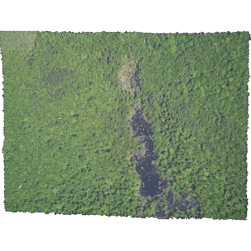
The black edges are not plotted.
Both data sets have
NoDatavalues, however, in the RGB_stack the NoData value is not defined in the tiff tags, thus R renders them as black as the reflectance values are 0. The black edges in the other file are defined as -9999 and R renders them as NA.
R
describe("data/NEON-DS-Airborne-Remote-Sensing/HARV/RGB_Imagery/HARV_RGB_Ortho.tif")
OUTPUT
 [1] "Driver: GTiff/GeoTIFF"
 [2] "Files: data/NEON-DS-Airborne-Remote-Sensing/HARV/RGB_Imagery/HARV_RGB_Ortho.tif"
 [3] "Size is 3073, 2317"
 [4] "Coordinate System is:"
 [5] "PROJCRS[\"WGS 84 / UTM zone 18N\","
 [6] "    BASEGEOGCRS[\"WGS 84\","
 [7] "        DATUM[\"World Geodetic System 1984\","
 [8] "            ELLIPSOID[\"WGS 84\",6378137,298.257223563,"
 [9] "                LENGTHUNIT[\"metre\",1]]],"
[10] "        PRIMEM[\"Greenwich\",0,"
[11] "            ANGLEUNIT[\"degree\",0.0174532925199433]],"
[12] "        ID[\"EPSG\",4326]],"
[13] "    CONVERSION[\"UTM zone 18N\","
[14] "        METHOD[\"Transverse Mercator\","
[15] "            ID[\"EPSG\",9807]],"
[16] "        PARAMETER[\"Latitude of natural origin\",0,"
[17] "            ANGLEUNIT[\"degree\",0.0174532925199433],"
[18] "            ID[\"EPSG\",8801]],"
[19] "        PARAMETER[\"Longitude of natural origin\",-75,"
[20] "            ANGLEUNIT[\"degree\",0.0174532925199433],"
[21] "            ID[\"EPSG\",8802]],"
[22] "        PARAMETER[\"Scale factor at natural origin\",0.9996,"
[23] "            SCALEUNIT[\"unity\",1],"
[24] "            ID[\"EPSG\",8805]],"
[25] "        PARAMETER[\"False easting\",500000,"
[26] "            LENGTHUNIT[\"metre\",1],"
[27] "            ID[\"EPSG\",8806]],"
[28] "        PARAMETER[\"False northing\",0,"
[29] "            LENGTHUNIT[\"metre\",1],"
[30] "            ID[\"EPSG\",8807]]],"
[31] "    CS[Cartesian,2],"
[32] "        AXIS[\"(E)\",east,"
[33] "            ORDER[1],"
[34] "            LENGTHUNIT[\"metre\",1]],"
[35] "        AXIS[\"(N)\",north,"
[36] "            ORDER[2],"
[37] "            LENGTHUNIT[\"metre\",1]],"
[38] "    USAGE["
[39] "        SCOPE[\"Engineering survey, topographic mapping.\"],"
[40] "        AREA[\"Between 78°W and 72°W, northern hemisphere between equator and 84°N, onshore and offshore. Bahamas. Canada - Nunavut; Ontario; Quebec. Colombia. Cuba. Ecuador. Greenland. Haiti. Jamica. Panama. Turks and Caicos Islands. United States (USA). Venezuela.\"],"
[41] "        BBOX[0,-78,84,-72]],"
[42] "    ID[\"EPSG\",32618]]"
[43] "Data axis to CRS axis mapping: 1,2"
[44] "Origin = (731998.500000000000000,4713535.500000000000000)"
[45] "Pixel Size = (0.250000000000000,-0.250000000000000)"
[46] "Metadata:"
[47] "  AREA_OR_POINT=Area"
[48] "Image Structure Metadata:"
[49] "  COMPRESSION=LZW"
[50] "  INTERLEAVE=PIXEL"
[51] "Corner Coordinates:"
[52] "Upper Left  (  731998.500, 4713535.500) ( 72d10'29.27\"W, 42d32'21.80\"N)"
[53] "Lower Left  (  731998.500, 4712956.250) ( 72d10'30.11\"W, 42d32' 3.04\"N)"
[54] "Upper Right (  732766.750, 4713535.500) ( 72d 9'55.63\"W, 42d32'20.97\"N)"
[55] "Lower Right (  732766.750, 4712956.250) ( 72d 9'56.48\"W, 42d32' 2.21\"N)"
[56] "Center      (  732382.625, 4713245.875) ( 72d10'12.87\"W, 42d32'12.00\"N)"
[57] "Band 1 Block=3073x1 Type=Float64, ColorInterp=Gray"
[58] "  Min=0.000 Max=255.000 "
[59] "  Minimum=0.000, Maximum=255.000, Mean=nan, StdDev=nan"
[60] "  NoData Value=-1.69999999999999994e+308"
[61] "  Metadata:"
[62] "    STATISTICS_MAXIMUM=255"
[63] "    STATISTICS_MEAN=nan"
[64] "    STATISTICS_MINIMUM=0"
[65] "    STATISTICS_STDDEV=nan"
[66] "Band 2 Block=3073x1 Type=Float64, ColorInterp=Undefined"
[67] "  Min=0.000 Max=255.000 "
[68] "  Minimum=0.000, Maximum=255.000, Mean=nan, StdDev=nan"
[69] "  NoData Value=-1.69999999999999994e+308"
[70] "  Metadata:"
[71] "    STATISTICS_MAXIMUM=255"
[72] "    STATISTICS_MEAN=nan"
[73] "    STATISTICS_MINIMUM=0"
[74] "    STATISTICS_STDDEV=nan"
[75] "Band 3 Block=3073x1 Type=Float64, ColorInterp=Undefined"
[76] "  Min=0.000 Max=255.000 "
[77] "  Minimum=0.000, Maximum=255.000, Mean=nan, StdDev=nan"
[78] "  NoData Value=-1.69999999999999994e+308"
[79] "  Metadata:"
[80] "    STATISTICS_MAXIMUM=255"
[81] "    STATISTICS_MEAN=nan"
[82] "    STATISTICS_MINIMUM=0"
[83] "    STATISTICS_STDDEV=nan"
Data Tip
We can create a raster object from several, individual single-band GeoTIFFs too. We will do this in a later episode, Raster Time Series Data in R.
SpatRaster in R
The R SpatRaster object type can handle rasters with multiple bands. The SpatRaster only holds parameters that describe the properties of raster data that is located somewhere on our computer.
A SpatRasterDataset object can hold references to sub-datasets, that is, SpatRaster objects. In most cases, we can work with a SpatRaster in the same way we might work with a SpatRasterDataset.
More Resources
You can read the help for the rast() and
sds() functions by typing ?rast or
?sds.
We can build a SpatRasterDataset using a SpatRaster or a list of SpatRaster:
R
RGB_sds_HARV <- sds(RGB_stack_HARV)
RGB_sds_HARV <- sds(list(RGB_stack_HARV, RGB_stack_HARV))
We can retrieve the SpatRaster objects from a SpatRasterDataset using subsetting:
R
RGB_sds_HARV[[1]]
OUTPUT
class       : SpatRaster
dimensions  : 2317, 3073, 3  (nrow, ncol, nlyr)
resolution  : 0.25, 0.25  (x, y)
extent      : 731998.5, 732766.8, 4712956, 4713536  (xmin, xmax, ymin, ymax)
coord. ref. : WGS 84 / UTM zone 18N (EPSG:32618)
source      : HARV_RGB_Ortho.tif
names       : HARV_RGB_Ortho_1, HARV_RGB_Ortho_2, HARV_RGB_Ortho_3
min values  :                0,                0,                0
max values  :              255,              255,              255
R
RGB_sds_HARV[[2]]
OUTPUT
class       : SpatRaster
dimensions  : 2317, 3073, 3  (nrow, ncol, nlyr)
resolution  : 0.25, 0.25  (x, y)
extent      : 731998.5, 732766.8, 4712956, 4713536  (xmin, xmax, ymin, ymax)
coord. ref. : WGS 84 / UTM zone 18N (EPSG:32618)
source      : HARV_RGB_Ortho.tif
names       : HARV_RGB_Ortho_1, HARV_RGB_Ortho_2, HARV_RGB_Ortho_3
min values  :                0,                0,                0
max values  :              255,              255,              255
Challenge: What Functions Can Be Used on an R Object of a particular class?
We can view various functions (or methods) available to use on an R
object with methods(class=class(objectNameHere)). Use this
to figure out:
- What methods can be used on the
RGB_stack_HARVobject? - What methods can be used on a single band within
RGB_stack_HARV? - Why do you think there isn’t a difference?
- We can see a list of all of the methods available for our RasterStack object:
R
methods(class=class(RGB_stack_HARV))
OUTPUT
  [1] !                     [                     [[
  [4] [[<-                  [<-                   %in%
  [7] $                     $<-                   activeCat
 [10] activeCat<-           add<-                 addCats
 [13] adjacent              aggregate             align
 [16] all.equal             allNA                 animate
 [19] anyNA                 app                   approximate
 [22] area                  Arith                 as.array
 [25] as.bool               as.character          as.contour
 [28] as.data.frame         as.factor             as.int
 [31] as.integer            as.lines              as.list
 [34] as.logical            as.matrix             as.numeric
 [37] as.points             as.polygons           as.raster
 [40] atan_2                atan2                 autocor
 [43] barplot               bestMatch             blocks
 [46] boundaries            boxplot               buffer
 [49] c                     catalyze              categories
 [52] cats                  cellFromRowCol        cellFromRowColCombine
 [55] cellFromXY            cells                 cellSize
 [58] clamp_ts              clamp                 classify
 [61] click                 coerce                colFromCell
 [64] colFromX              colorize              coltab
 [67] coltab<-              Compare               compare
 [70] compareGeom           concats               contour
 [73] costDist              countNA               cover
 [76] crds                  crop                  crosstab
 [79] crs                   crs<-                 datatype
 [82] deepcopy              density               depth
 [85] depth<-               diff                  dim
 [88] dim<-                 direction             disagg
 [91] distance              droplevels            expanse
 [94] ext                   ext<-                 extend
 [97] extract               extractRange          fillTime
[100] flip                  focal                 focal3D
[103] focalCor              focalCpp              focalPairs
[106] focalReg              focalValues           freq
[109] getTileExtents        global                gridDist
[112] gridDistance          has.colors            has.RGB
[115] has.time              hasMinMax             hasValues
[118] head                  hist                  identical
[121] ifel                  image                 init
[124] inMemory              inset                 interpIDW
[127] interpNear            interpolate           intersect
[130] is.bool               is.factor             is.finite
[133] is.infinite           is.int                is.lonlat
[136] is.na                 is.nan                is.related
[139] is.rotated            isFALSE               isTRUE
[142] k_means               lapp                  layerCor
[145] levels                levels<-              linearUnits
[148] lines                 log                   Logic
[151] logic                 longnames             longnames<-
[154] makeTiles             mask                  match
[157] math                  Math                  Math2
[160] mean                  median                merge
[163] meta                  metags                metags<-
[166] minmax                modal                 mosaic
[169] NAflag                NAflag<-              names
[172] names<-               ncell                 ncol
[175] ncol<-                nlyr                  nlyr<-
[178] noNA                  not.na                nrow
[181] nrow<-                nsrc                  origin
[184] origin<-              pairs                 panel
[187] patches               persp                 plet
[190] plot                  plotRGB               points
[193] polys                 prcomp                predict
[196] princomp              project               quantile
[199] rangeFill             rapp                  rast
[202] rasterize             rasterizeGeom         rasterizeWin
[205] rcl                   readStart             readStop
[208] readValues            rectify               regress
[211] relate                rep                   res
[214] res<-                 resample              rescale
[217] rev                   RGB                   RGB<-
[220] roll                  rotate                rowColCombine
[223] rowColFromCell        rowFromCell           rowFromY
[226] sapp                  saveRDS               scale
[229] scoff                 scoff<-               sds
[232] segregate             sel                   selectHighest
[235] selectRange           serialize             set.cats
[238] set.crs               set.ext               set.names
[241] set.RGB               set.values            setMinMax
[244] setValues             shift                 show
[247] sieve                 size                  sort
[250] sources               spatSample            split
[253] sprc                  stdev                 str
[256] stretch               subset                subst
[259] summary               Summary               t
[262] tail                  tapp                  terrain
[265] text                  tighten               time
[268] time<-                timeInfo              trans
[271] trim                  unique                units
[274] units<-               update                values
[277] values<-              varnames              varnames<-
[280] viewshed              weighted.mean         where.max
[283] where.min             which.lyr             which.max
[286] which.min             window                window<-
[289] wrap                  wrapCache             writeCDF
[292] writeRaster           writeStart            writeStop
[295] writeValues           xapp                  xFromCell
[298] xFromCol              xmax                  xmax<-
[301] xmin                  xmin<-                xres
[304] xyFromCell            yFromCell             yFromRow
[307] ymax                  ymax<-                ymin
[310] ymin<-                yres                  zonal
[313] zoom
see '?methods' for accessing help and source code- And compare that with the methods available for a single band:
R
methods(class=class(RGB_stack_HARV[[1]]))
OUTPUT
  [1] !                     [                     [[
  [4] [[<-                  [<-                   %in%
  [7] $                     $<-                   activeCat
 [10] activeCat<-           add<-                 addCats
 [13] adjacent              aggregate             align
 [16] all.equal             allNA                 animate
 [19] anyNA                 app                   approximate
 [22] area                  Arith                 as.array
 [25] as.bool               as.character          as.contour
 [28] as.data.frame         as.factor             as.int
 [31] as.integer            as.lines              as.list
 [34] as.logical            as.matrix             as.numeric
 [37] as.points             as.polygons           as.raster
 [40] atan_2                atan2                 autocor
 [43] barplot               bestMatch             blocks
 [46] boundaries            boxplot               buffer
 [49] c                     catalyze              categories
 [52] cats                  cellFromRowCol        cellFromRowColCombine
 [55] cellFromXY            cells                 cellSize
 [58] clamp_ts              clamp                 classify
 [61] click                 coerce                colFromCell
 [64] colFromX              colorize              coltab
 [67] coltab<-              Compare               compare
 [70] compareGeom           concats               contour
 [73] costDist              countNA               cover
 [76] crds                  crop                  crosstab
 [79] crs                   crs<-                 datatype
 [82] deepcopy              density               depth
 [85] depth<-               diff                  dim
 [88] dim<-                 direction             disagg
 [91] distance              droplevels            expanse
 [94] ext                   ext<-                 extend
 [97] extract               extractRange          fillTime
[100] flip                  focal                 focal3D
[103] focalCor              focalCpp              focalPairs
[106] focalReg              focalValues           freq
[109] getTileExtents        global                gridDist
[112] gridDistance          has.colors            has.RGB
[115] has.time              hasMinMax             hasValues
[118] head                  hist                  identical
[121] ifel                  image                 init
[124] inMemory              inset                 interpIDW
[127] interpNear            interpolate           intersect
[130] is.bool               is.factor             is.finite
[133] is.infinite           is.int                is.lonlat
[136] is.na                 is.nan                is.related
[139] is.rotated            isFALSE               isTRUE
[142] k_means               lapp                  layerCor
[145] levels                levels<-              linearUnits
[148] lines                 log                   Logic
[151] logic                 longnames             longnames<-
[154] makeTiles             mask                  match
[157] math                  Math                  Math2
[160] mean                  median                merge
[163] meta                  metags                metags<-
[166] minmax                modal                 mosaic
[169] NAflag                NAflag<-              names
[172] names<-               ncell                 ncol
[175] ncol<-                nlyr                  nlyr<-
[178] noNA                  not.na                nrow
[181] nrow<-                nsrc                  origin
[184] origin<-              pairs                 panel
[187] patches               persp                 plet
[190] plot                  plotRGB               points
[193] polys                 prcomp                predict
[196] princomp              project               quantile
[199] rangeFill             rapp                  rast
[202] rasterize             rasterizeGeom         rasterizeWin
[205] rcl                   readStart             readStop
[208] readValues            rectify               regress
[211] relate                rep                   res
[214] res<-                 resample              rescale
[217] rev                   RGB                   RGB<-
[220] roll                  rotate                rowColCombine
[223] rowColFromCell        rowFromCell           rowFromY
[226] sapp                  saveRDS               scale
[229] scoff                 scoff<-               sds
[232] segregate             sel                   selectHighest
[235] selectRange           serialize             set.cats
[238] set.crs               set.ext               set.names
[241] set.RGB               set.values            setMinMax
[244] setValues             shift                 show
[247] sieve                 size                  sort
[250] sources               spatSample            split
[253] sprc                  stdev                 str
[256] stretch               subset                subst
[259] summary               Summary               t
[262] tail                  tapp                  terrain
[265] text                  tighten               time
[268] time<-                timeInfo              trans
[271] trim                  unique                units
[274] units<-               update                values
[277] values<-              varnames              varnames<-
[280] viewshed              weighted.mean         where.max
[283] where.min             which.lyr             which.max
[286] which.min             window                window<-
[289] wrap                  wrapCache             writeCDF
[292] writeRaster           writeStart            writeStop
[295] writeValues           xapp                  xFromCell
[298] xFromCol              xmax                  xmax<-
[301] xmin                  xmin<-                xres
[304] xyFromCell            yFromCell             yFromRow
[307] ymax                  ymax<-                ymin
[310] ymin<-                yres                  zonal
[313] zoom
see '?methods' for accessing help and source code- A SpatRaster is the same no matter its number of bands.
Key Points
- A single raster file can contain multiple bands or layers.
- Use the
rast()function to load all bands in a multi-layer raster file into R. - Individual bands within a SpatRaster can be accessed, analyzed, and visualized using the same functions no matter how many bands it holds.
Content from Open and Plot Vector Layers
Last updated on 2024-10-15 | Edit this page
Overview
Questions
- How can I distinguish between and visualize point, line and polygon vector data?
Objectives
- Know the difference between point, line, and polygon vector elements.
- Load point, line, and polygon vector layers into R.
- Access the attributes of a spatial object in R.
Things You’ll Need To Complete This Episode
See the lesson homepage for detailed information about the software, data, and other prerequisites you will need to work through the examples in this episode.
Starting with this episode, we will be moving from working with
raster data to working with vector data. In this episode, we will open
and plot point, line and polygon vector data loaded from ESRI’s
shapefile format into R. These data refer to the NEON
Harvard Forest field site, which we have been working with in
previous episodes. In later episodes, we will learn how to work with
raster and vector data together and combine them into a single plot.
Import Vector Data
We will use the sf package to work with vector data in
R. We will also use the terra package, which has been
loaded in previous episodes, so we can explore raster and vector spatial
metadata using similar commands. Make sure you have the sf
library loaded.
R
library(sf)
The vector layers that we will import from ESRI’s
shapefile format are:
- A polygon vector layer representing our field site boundary,
- A line vector layer representing roads, and
- A point vector layer representing the location of the Fisher flux tower located at the NEON Harvard Forest field site.
The first vector layer that we will open contains the boundary of our
study area (or our Area Of Interest or AOI, hence the name
aoiBoundary). To import a vector layer from an ESRI
shapefile we use the sf function
st_read(). st_read() requires the file path to
the ESRI shapefile.
Let’s import our AOI:
R
aoi_boundary_HARV <- st_read(
  "data/NEON-DS-Site-Layout-Files/HARV/HarClip_UTMZ18.shp")
OUTPUT
Reading layer `HarClip_UTMZ18' from data source
  `/home/runner/work/r-raster-vector-geospatial/r-raster-vector-geospatial/site/built/data/NEON-DS-Site-Layout-Files/HARV/HarClip_UTMZ18.shp'
  using driver `ESRI Shapefile'
Simple feature collection with 1 feature and 1 field
Geometry type: POLYGON
Dimension:     XY
Bounding box:  xmin: 732128 ymin: 4713209 xmax: 732251.1 ymax: 4713359
Projected CRS: WGS 84 / UTM zone 18N
Vector Layer Metadata & Attributes
When we import the HarClip_UTMZ18 vector layer from an
ESRI shapefile into R (as our
aoi_boundary_HARV object), the st_read()
function automatically stores information about the data. We are
particularly interested in the geospatial metadata, describing the
format, CRS, extent, and other components of the vector data, and the
attributes which describe properties associated with each individual
vector object.
Data Tip
The Explore and Plot by Vector Layer Attributes episode provides more information on both metadata and attributes and using attributes to subset and plot data.
Spatial Metadata
Key metadata for all vector layers includes:
- Object Type: the class of the imported object.
- Coordinate Reference System (CRS): the projection of the data.
- Extent: the spatial extent (i.e. geographic area that the vector layer covers) of the data. Note that the spatial extent for a vector layer represents the combined extent for all individual objects in the vector layer.
We can view metadata of a vector layer using the
st_geometry_type(), st_crs() and
st_bbox() functions. First, let’s view the geometry type
for our AOI vector layer:
R
st_geometry_type(aoi_boundary_HARV)
OUTPUT
[1] POLYGON
18 Levels: GEOMETRY POINT LINESTRING POLYGON MULTIPOINT ... TRIANGLE
Our aoi_boundary_HARV is a polygon spatial object. The
18 levels shown below our output list the possible categories of the
geometry type. Now let’s check what CRS this file data is in:
R
st_crs(aoi_boundary_HARV)
OUTPUT
Coordinate Reference System:
  User input: WGS 84 / UTM zone 18N
  wkt:
PROJCRS["WGS 84 / UTM zone 18N",
    BASEGEOGCRS["WGS 84",
        DATUM["World Geodetic System 1984",
            ELLIPSOID["WGS 84",6378137,298.257223563,
                LENGTHUNIT["metre",1]]],
        PRIMEM["Greenwich",0,
            ANGLEUNIT["degree",0.0174532925199433]],
        ID["EPSG",4326]],
    CONVERSION["UTM zone 18N",
        METHOD["Transverse Mercator",
            ID["EPSG",9807]],
        PARAMETER["Latitude of natural origin",0,
            ANGLEUNIT["Degree",0.0174532925199433],
            ID["EPSG",8801]],
        PARAMETER["Longitude of natural origin",-75,
            ANGLEUNIT["Degree",0.0174532925199433],
            ID["EPSG",8802]],
        PARAMETER["Scale factor at natural origin",0.9996,
            SCALEUNIT["unity",1],
            ID["EPSG",8805]],
        PARAMETER["False easting",500000,
            LENGTHUNIT["metre",1],
            ID["EPSG",8806]],
        PARAMETER["False northing",0,
            LENGTHUNIT["metre",1],
            ID["EPSG",8807]]],
    CS[Cartesian,2],
        AXIS["(E)",east,
            ORDER[1],
            LENGTHUNIT["metre",1]],
        AXIS["(N)",north,
            ORDER[2],
            LENGTHUNIT["metre",1]],
    ID["EPSG",32618]]
Our data in the CRS UTM zone 18N. The CRS is
critical to interpreting the spatial object’s extent values as it
specifies units. To find the extent of our AOI, we can use the
st_bbox() function:
R
st_bbox(aoi_boundary_HARV)
OUTPUT
     xmin      ymin      xmax      ymax
 732128.0 4713208.7  732251.1 4713359.2
The spatial extent of a vector layer or R spatial object represents the geographic “edge” or location that is the furthest north, south east and west. Thus it represents the overall geographic coverage of the spatial object. Image Source: National Ecological Observatory Network (NEON).
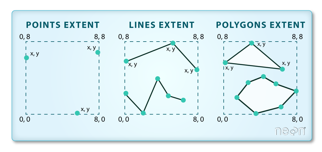
Lastly, we can view all of the metadata and attributes for this R spatial object by printing it to the screen:
R
aoi_boundary_HARV
OUTPUT
Simple feature collection with 1 feature and 1 field
Geometry type: POLYGON
Dimension:     XY
Bounding box:  xmin: 732128 ymin: 4713209 xmax: 732251.1 ymax: 4713359
Projected CRS: WGS 84 / UTM zone 18N
  id                       geometry
1  1 POLYGON ((732128 4713359, 7...
Spatial Data Attributes
We introduced the idea of spatial data attributes in an earlier lesson. Now we will explore how to use spatial data attributes stored in our data to plot different features.
Plot a vector layer
Next, let’s visualize the data in our sf object using
the ggplot package. Unlike with raster data, we do not need
to convert vector data to a dataframe before plotting with
ggplot.
We’re going to customize our boundary plot by setting the size,
color, and fill for our plot. When plotting sf objects with
ggplot2, you need to use the coord_sf()
coordinate system.
R
ggplot() +
  geom_sf(data = aoi_boundary_HARV, size = 3, color = "black", fill = "cyan1") +
  ggtitle("AOI Boundary Plot") +
  coord_sf()
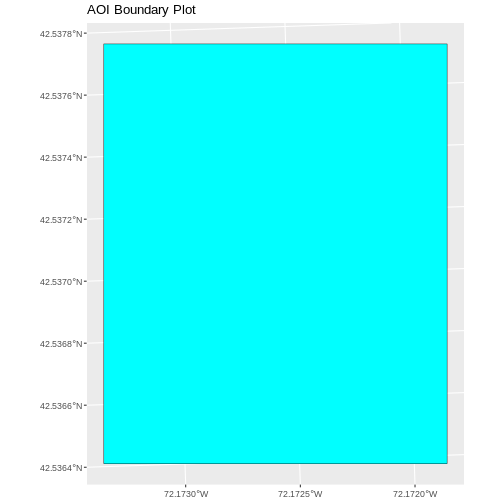
Challenge: Import Line and Point Vector Layers
Using the steps above, import the HARV_roads and HARVtower_UTM18N
vector layers into R. Call the HARV_roads object lines_HARV
and the HARVtower_UTM18N point_HARV.
Answer the following questions:
What type of R spatial object is created when you import each layer?
What is the CRS and extent for each object?
Do the files contain points, lines, or polygons?
How many spatial objects are in each file?
First we import the data:
R
lines_HARV <- st_read("data/NEON-DS-Site-Layout-Files/HARV/HARV_roads.shp")
OUTPUT
Reading layer `HARV_roads' from data source
  `/home/runner/work/r-raster-vector-geospatial/r-raster-vector-geospatial/site/built/data/NEON-DS-Site-Layout-Files/HARV/HARV_roads.shp'
  using driver `ESRI Shapefile'
Simple feature collection with 13 features and 15 fields
Geometry type: MULTILINESTRING
Dimension:     XY
Bounding box:  xmin: 730741.2 ymin: 4711942 xmax: 733295.5 ymax: 4714260
Projected CRS: WGS 84 / UTM zone 18N
R
point_HARV <- st_read("data/NEON-DS-Site-Layout-Files/HARV/HARVtower_UTM18N.shp")
OUTPUT
Reading layer `HARVtower_UTM18N' from data source
  `/home/runner/work/r-raster-vector-geospatial/r-raster-vector-geospatial/site/built/data/NEON-DS-Site-Layout-Files/HARV/HARVtower_UTM18N.shp'
  using driver `ESRI Shapefile'
Simple feature collection with 1 feature and 14 fields
Geometry type: POINT
Dimension:     XY
Bounding box:  xmin: 732183.2 ymin: 4713265 xmax: 732183.2 ymax: 4713265
Projected CRS: WGS 84 / UTM zone 18N
Then we check its class:
R
class(lines_HARV)
OUTPUT
[1] "sf" "data.frame"R
class(point_HARV)
OUTPUT
[1] "sf" "data.frame"We also check the CRS and extent of each object:
R
st_crs(lines_HARV)
OUTPUT
Coordinate Reference System:
  User input: WGS 84 / UTM zone 18N
  wkt:
PROJCRS["WGS 84 / UTM zone 18N",
    BASEGEOGCRS["WGS 84",
        DATUM["World Geodetic System 1984",
            ELLIPSOID["WGS 84",6378137,298.257223563,
                LENGTHUNIT["metre",1]]],
        PRIMEM["Greenwich",0,
            ANGLEUNIT["degree",0.0174532925199433]],
        ID["EPSG",4326]],
    CONVERSION["UTM zone 18N",
        METHOD["Transverse Mercator",
            ID["EPSG",9807]],
        PARAMETER["Latitude of natural origin",0,
            ANGLEUNIT["Degree",0.0174532925199433],
            ID["EPSG",8801]],
        PARAMETER["Longitude of natural origin",-75,
            ANGLEUNIT["Degree",0.0174532925199433],
            ID["EPSG",8802]],
        PARAMETER["Scale factor at natural origin",0.9996,
            SCALEUNIT["unity",1],
            ID["EPSG",8805]],
        PARAMETER["False easting",500000,
            LENGTHUNIT["metre",1],
            ID["EPSG",8806]],
        PARAMETER["False northing",0,
            LENGTHUNIT["metre",1],
            ID["EPSG",8807]]],
    CS[Cartesian,2],
        AXIS["(E)",east,
            ORDER[1],
            LENGTHUNIT["metre",1]],
        AXIS["(N)",north,
            ORDER[2],
            LENGTHUNIT["metre",1]],
    ID["EPSG",32618]]
R
st_bbox(lines_HARV)
OUTPUT
     xmin      ymin      xmax      ymax
 730741.2 4711942.0  733295.5 4714260.0
R
st_crs(point_HARV)
OUTPUT
Coordinate Reference System:
  User input: WGS 84 / UTM zone 18N
  wkt:
PROJCRS["WGS 84 / UTM zone 18N",
    BASEGEOGCRS["WGS 84",
        DATUM["World Geodetic System 1984",
            ELLIPSOID["WGS 84",6378137,298.257223563,
                LENGTHUNIT["metre",1]]],
        PRIMEM["Greenwich",0,
            ANGLEUNIT["degree",0.0174532925199433]],
        ID["EPSG",4326]],
    CONVERSION["UTM zone 18N",
        METHOD["Transverse Mercator",
            ID["EPSG",9807]],
        PARAMETER["Latitude of natural origin",0,
            ANGLEUNIT["Degree",0.0174532925199433],
            ID["EPSG",8801]],
        PARAMETER["Longitude of natural origin",-75,
            ANGLEUNIT["Degree",0.0174532925199433],
            ID["EPSG",8802]],
        PARAMETER["Scale factor at natural origin",0.9996,
            SCALEUNIT["unity",1],
            ID["EPSG",8805]],
        PARAMETER["False easting",500000,
            LENGTHUNIT["metre",1],
            ID["EPSG",8806]],
        PARAMETER["False northing",0,
            LENGTHUNIT["metre",1],
            ID["EPSG",8807]]],
    CS[Cartesian,2],
        AXIS["(E)",east,
            ORDER[1],
            LENGTHUNIT["metre",1]],
        AXIS["(N)",north,
            ORDER[2],
            LENGTHUNIT["metre",1]],
    ID["EPSG",32618]]
R
st_bbox(point_HARV)
OUTPUT
     xmin      ymin      xmax      ymax
 732183.2 4713265.0  732183.2 4713265.0
To see the number of objects in each file, we can look at the output
from when we read these objects into R. lines_HARV contains
13 features (all lines) and point_HARV contains only one
point.
Key Points
- Metadata for vector layers include geometry type, CRS, and extent.
- Load spatial objects into R with the
st_read()function. - Spatial objects can be plotted directly with
ggplotusing thegeom_sf()function. No need to convert to a dataframe.
Content from Explore and Plot by Vector Layer Attributes
Last updated on 2024-10-15 | Edit this page
Overview
Questions
- How can I compute on the attributes of a spatial object?
Objectives
- Query attributes of a spatial object.
- Subset spatial objects using specific attribute values.
- Plot a vector feature, colored by unique attribute values.
Things You’ll Need To Complete This Episode
See the lesson homepage for detailed information about the software, data, and other prerequisites you will need to work through the examples in this episode.
This episode continues our discussion of vector layer attributes and covers how to work with vector layer attributes in R. It covers how to identify and query layer attributes, as well as how to subset features by specific attribute values. Finally, we will learn how to plot a feature according to a set of attribute values.
Load the Data
We will continue using the sf, terra and
ggplot2 packages in this episode. Make sure that you have
these packages loaded. We will continue to work with the three ESRI
shapefiles (vector layers) that we loaded in the Open and Plot Vector Layers in
R episode.
Query Vector Feature Metadata
As we discussed in the Open and Plot Vector Layers in R episode, we can view metadata associated with an R object using:
-
st_geometry_type()- The type of vector data stored in the object. -
nrow()- The number of features in the object -
st_bbox()- The spatial extent (geographic area covered by) of the object. -
st_crs()- The CRS (spatial projection) of the data.
We started to explore our point_HARV object in the
previous episode. To see a summary of all of the metadata associated
with our point_HARV object, we can view the object with
View(point_HARV) or print a summary of the object itself to
the console.
R
point_HARV
OUTPUT
Simple feature collection with 1 feature and 14 fields
Geometry type: POINT
Dimension:     XY
Bounding box:  xmin: 732183.2 ymin: 4713265 xmax: 732183.2 ymax: 4713265
Projected CRS: WGS 84 / UTM zone 18N
  Un_ID Domain DomainName       SiteName Type       Sub_Type     Lat      Long
1     A      1  Northeast Harvard Forest Core Advanced Tower 42.5369 -72.17266
  Zone  Easting Northing                Ownership    County annotation
1   18 732183.2  4713265 Harvard University, LTER Worcester         C1
                  geometry
1 POINT (732183.2 4713265)
We can use the ncol function to count the number of
attributes associated with a spatial object too. Note that the geometry
is just another column and counts towards the total.
R
ncol(lines_HARV)
OUTPUT
[1] 16We can view the individual name of each attribute using the
names() function in R:
R
names(lines_HARV)
OUTPUT
 [1] "OBJECTID_1" "OBJECTID"   "TYPE"       "NOTES"      "MISCNOTES"
 [6] "RULEID"     "MAPLABEL"   "SHAPE_LENG" "LABEL"      "BIKEHORSE"
[11] "RESVEHICLE" "RECMAP"     "Shape_Le_1" "ResVehic_1" "BicyclesHo"
[16] "geometry"
We could also view just the first 6 rows of attribute values using
the head() function to get a preview of the data:
R
head(lines_HARV)
OUTPUT
Simple feature collection with 6 features and 15 fields
Geometry type: MULTILINESTRING
Dimension:     XY
Bounding box:  xmin: 730741.2 ymin: 4712685 xmax: 732232.3 ymax: 4713726
Projected CRS: WGS 84 / UTM zone 18N
  OBJECTID_1 OBJECTID       TYPE             NOTES MISCNOTES RULEID
1         14       48 woods road Locust Opening Rd      <NA>      5
2         40       91   footpath              <NA>      <NA>      6
3         41      106   footpath              <NA>      <NA>      6
4        211      279 stone wall              <NA>      <NA>      1
5        212      280 stone wall              <NA>      <NA>      1
6        213      281 stone wall              <NA>      <NA>      1
           MAPLABEL SHAPE_LENG             LABEL BIKEHORSE RESVEHICLE RECMAP
1 Locust Opening Rd 1297.35706 Locust Opening Rd         Y         R1      Y
2              <NA>  146.29984              <NA>         Y         R1      Y
3              <NA>  676.71804              <NA>         Y         R2      Y
4              <NA>  231.78957              <NA>      <NA>       <NA>   <NA>
5              <NA>   45.50864              <NA>      <NA>       <NA>   <NA>
6              <NA>  198.39043              <NA>      <NA>       <NA>   <NA>
  Shape_Le_1                            ResVehic_1                  BicyclesHo
1 1297.10617    R1 - All Research Vehicles Allowed Bicycles and Horses Allowed
2  146.29983    R1 - All Research Vehicles Allowed Bicycles and Horses Allowed
3  676.71807 R2 - 4WD/High Clearance Vehicles Only Bicycles and Horses Allowed
4  231.78962                                  <NA>                        <NA>
5   45.50859                                  <NA>                        <NA>
6  198.39041                                  <NA>                        <NA>
                        geometry
1 MULTILINESTRING ((730819.2 ...
2 MULTILINESTRING ((732040.2 ...
3 MULTILINESTRING ((732057 47...
4 MULTILINESTRING ((731903.6 ...
5 MULTILINESTRING ((732039.1 ...
6 MULTILINESTRING ((732056.2 ...
Challenge: Attributes for Different Spatial Classes
Explore the attributes associated with the point_HARV
and aoi_boundary_HARV spatial objects.
How many attributes does each have?
Who owns the site in the
point_HARVdata object?Which of the following is NOT an attribute of the
point_HARVdata object?
- Latitude B) County C) Country
- To find the number of attributes, we use the
ncol()function:
R
ncol(point_HARV)
OUTPUT
[1] 15R
ncol(aoi_boundary_HARV)
OUTPUT
[1] 2- Ownership information is in a column named
Ownership:
R
point_HARV$Ownership
OUTPUT
[1] "Harvard University, LTER"- To see a list of all of the attributes, we can use the
names()function:
R
names(point_HARV)
OUTPUT
 [1] "Un_ID"      "Domain"     "DomainName" "SiteName"   "Type"
 [6] "Sub_Type"   "Lat"        "Long"       "Zone"       "Easting"
[11] "Northing"   "Ownership"  "County"     "annotation" "geometry"
“Country” is not an attribute of this object.
Explore Values within One Attribute
We can explore individual values stored within a particular
attribute. Comparing attributes to a spreadsheet or a data frame, this
is similar to exploring values in a column. We did this with the
gapminder dataframe in an
earlier lesson. For spatial objects, we can use the same syntax:
objectName$attributeName.
We can see the contents of the TYPE field of our lines
feature:
R
lines_HARV$TYPE
OUTPUT
 [1] "woods road" "footpath"   "footpath"   "stone wall" "stone wall"
 [6] "stone wall" "stone wall" "stone wall" "stone wall" "boardwalk"
[11] "woods road" "woods road" "woods road"
To see only unique values within the TYPE field, we can
use the unique() function for extracting the possible
values of a character variable (R also is able to handle categorical
variables called factors; we worked with factors a little bit in an
earlier lesson.
R
unique(lines_HARV$TYPE)
OUTPUT
[1] "woods road" "footpath" "stone wall" "boardwalk" Subset Features
We can use the filter() function from dplyr
that we worked with in an earlier
lesson to select a subset of features from a spatial object in R,
just like with data frames.
For example, we might be interested only in features that are of
TYPE “footpath”. Once we subset out this data, we can use
it as input to other code so that code only operates on the footpath
lines.
R
footpath_HARV <- lines_HARV %>%
  filter(TYPE == "footpath")
nrow(footpath_HARV)
OUTPUT
[1] 2Our subsetting operation reduces the features count to
2. This means that only two feature lines in our spatial object have the
attribute TYPE == footpath. We can plot only the footpath
lines:
R
ggplot() +
  geom_sf(data = footpath_HARV) +
  ggtitle("NEON Harvard Forest Field Site", subtitle = "Footpaths") +
  coord_sf()
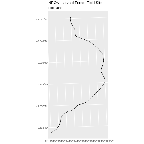
There are two features in our footpaths subset. Why does the plot
look like there is only one feature? Let’s adjust the colors used in our
plot. If we have 2 features in our vector object, we can plot each using
a unique color by assigning a column name to the color aesthetic
(color =). We use the syntax aes(color = ) to
do this. We can also alter the default line thickness by using the
size = parameter, as the default value of 0.5 can be hard
to see. Note that size is placed outside of the aes()
function, as we are not connecting line thickness to a data
variable.
R
ggplot() +
  geom_sf(data = footpath_HARV, aes(color = factor(OBJECTID)), size = 1.5) +
  labs(color = 'Footpath ID') +
  ggtitle("NEON Harvard Forest Field Site", subtitle = "Footpaths") +
  coord_sf()
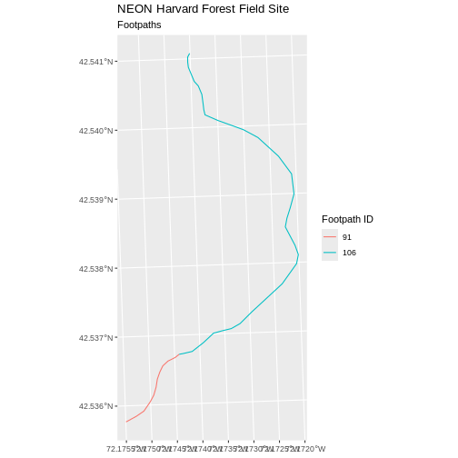
Now, we see that there are in fact two features in our plot!
Challenge: Subset Spatial Line Objects Part 1
Subset out all boardwalk from the lines layer and plot
it.
First we will save an object with only the boardwalk lines:
R
boardwalk_HARV <- lines_HARV %>%
  filter(TYPE == "boardwalk")
Let’s check how many features there are in this subset:
R
nrow(boardwalk_HARV)
OUTPUT
[1] 1Now let’s plot that data:
R
ggplot() +
  geom_sf(data = boardwalk_HARV, size = 1.5) +
  ggtitle("NEON Harvard Forest Field Site", subtitle = "Boardwalks") +
  coord_sf()
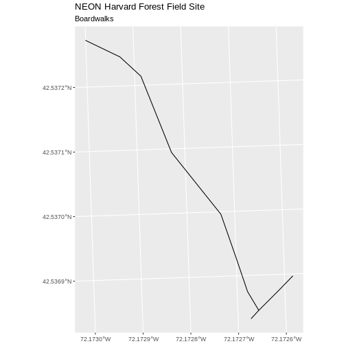
Challenge: Subset Spatial Line Objects Part 2
Subset out all stone wall features from the lines layer
and plot it. For each plot, color each feature using a unique color.
First we will save an object with only the stone wall lines and check the number of features:
R
stoneWall_HARV <- lines_HARV %>%
  filter(TYPE == "stone wall")
nrow(stoneWall_HARV)
OUTPUT
[1] 6Now we can plot the data:
R
ggplot() +
  geom_sf(data = stoneWall_HARV, aes(color = factor(OBJECTID)), size = 1.5) +
  labs(color = 'Wall ID') +
  ggtitle("NEON Harvard Forest Field Site", subtitle = "Stonewalls") +
  coord_sf()
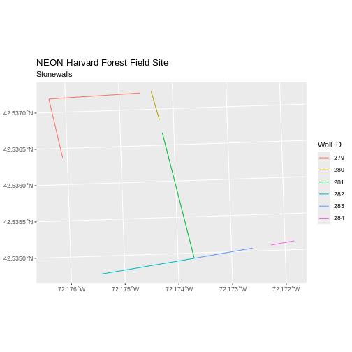
Customize Plots
In the examples above, ggplot() automatically selected
colors for each line based on a default color order. If we don’t like
those default colors, we can create a vector of colors - one for each
feature.
First we will check how many unique levels our factor has:
R
unique(lines_HARV$TYPE)
OUTPUT
[1] "woods road" "footpath" "stone wall" "boardwalk" Then we can create a palette of four colors, one for each feature in our vector object.
R
road_colors <- c("blue", "green", "navy", "purple")
We can tell ggplot to use these colors when we plot the
data.
R
ggplot() +
  geom_sf(data = lines_HARV, aes(color = TYPE)) +
  scale_color_manual(values = road_colors) +
  labs(color = 'Road Type') +
  ggtitle("NEON Harvard Forest Field Site", subtitle = "Roads & Trails") +
  coord_sf()
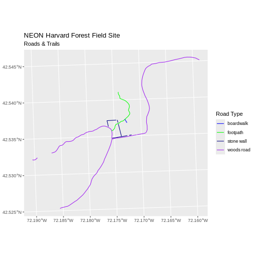
Adjust Line Width
We adjusted line width universally earlier. If we want a unique line width for each level or attribute category in our spatial object, we can use the same syntax that we used for colors, above.
We already know that we have four different TYPEs in the
lines_HARV object, so we will set four different line widths.
R
line_widths <- c(1, 2, 3, 4)
We can use those line widths when we plot the data.
R
ggplot() +
  geom_sf(data = lines_HARV, aes(color = TYPE, size = TYPE)) +
  scale_color_manual(values = road_colors) +
  labs(color = 'Road Type') +
  scale_size_manual(values = line_widths) +
  ggtitle("NEON Harvard Forest Field Site",
          subtitle = "Roads & Trails - Line width varies") +
  coord_sf()
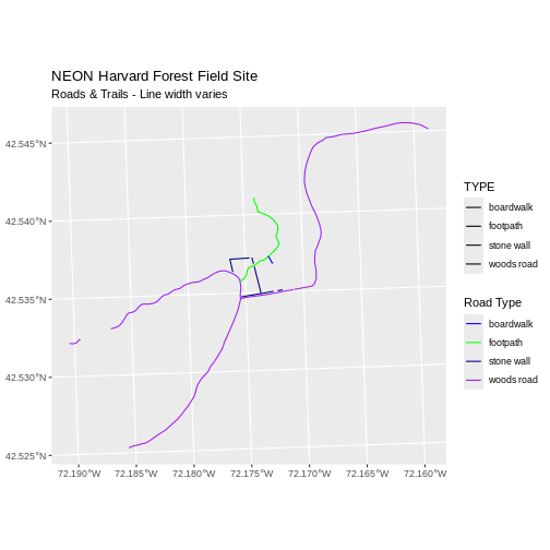
Challenge: Plot Line Width by Attribute
In the example above, we set the line widths to be 1, 2, 3, and 4. Because R orders alphabetically by default, this gave us a plot where woods roads (the last type) were the thickest and boardwalks were the thinnest.
Let’s create another plot where we show the different line types with the following thicknesses:
- woods road size = 6
- boardwalks size = 1
- footpath size = 3
- stone wall size = 2
First we need to look at the levels of our factor to see what order the road types are in:
R
unique(lines_HARV$TYPE)
OUTPUT
[1] "woods road" "footpath" "stone wall" "boardwalk" We then can create our line_width vector setting each of
the levels to the desired thickness.
R
line_width <- c(1, 3, 2, 6)
Now we can create our plot.
R
ggplot() +
  geom_sf(data = lines_HARV, aes(size = TYPE)) +
  scale_size_manual(values = line_width) +
  ggtitle("NEON Harvard Forest Field Site",
          subtitle = "Roads & Trails - Line width varies") +
  coord_sf()
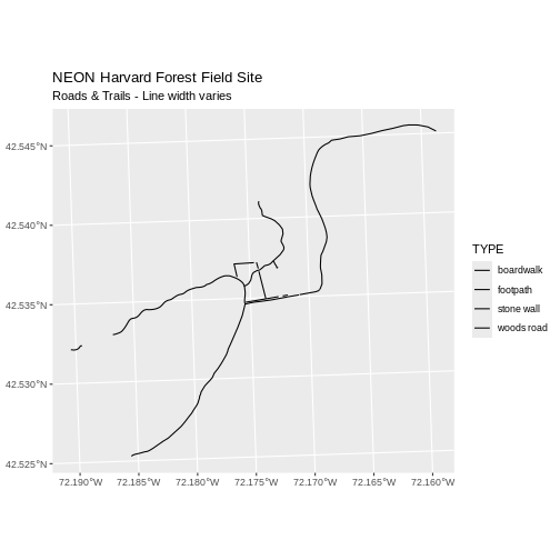
Add Plot Legend
We can add a legend to our plot too. When we add a legend, we use the following elements to specify labels and colors:
-
bottomright: We specify the location of our legend by using a default keyword. We could also usetop,topright, etc. -
levels(objectName$attributeName): Label the legend elements using the categories of levels in an attribute (e.g., levels(lines_HARV$TYPE) means use the levels boardwalk, footpath, etc). -
fill =: apply unique colors to the boxes in our legend.palette()is the default set of colors that R applies to all plots.
Let’s add a legend to our plot. We will use the
road_colors object that we created above to color the
legend. We can customize the appearance of our legend by manually
setting different parameters.
R
ggplot() +
  geom_sf(data = lines_HARV, aes(color = TYPE), size = 1.5) +
  scale_color_manual(values = road_colors) +
  labs(color = 'Road Type') +
  ggtitle("NEON Harvard Forest Field Site",
          subtitle = "Roads & Trails - Default Legend") +
  coord_sf()
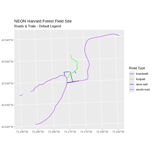
We can change the appearance of our legend by manually setting different parameters.
-
legend.text: change the font size -
legend.box.background: add an outline box
R
ggplot() +
  geom_sf(data = lines_HARV, aes(color = TYPE), size = 1.5) +
  scale_color_manual(values = road_colors) +
  labs(color = 'Road Type') +
  theme(legend.text = element_text(size = 20),
        legend.box.background = element_rect(size = 1)) +
  ggtitle("NEON Harvard Forest Field Site",
          subtitle = "Roads & Trails - Modified Legend") +
  coord_sf()
WARNING
Warning: The `size` argument of `element_rect()` is deprecated as of ggplot2 3.4.0.
ℹ Please use the `linewidth` argument instead.
This warning is displayed once every 8 hours.
Call `lifecycle::last_lifecycle_warnings()` to see where this warning was
generated.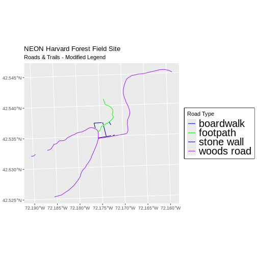
R
new_colors <- c("springgreen", "blue", "magenta", "orange")

ggplot() +
  geom_sf(data = lines_HARV, aes(color = TYPE), size = 1.5) +
  scale_color_manual(values = new_colors) +
  labs(color = 'Road Type') +
  theme(legend.text = element_text(size = 20),
        legend.box.background = element_rect(size = 1)) +
  ggtitle("NEON Harvard Forest Field Site",
          subtitle = "Roads & Trails - Pretty Colors") +
  coord_sf()
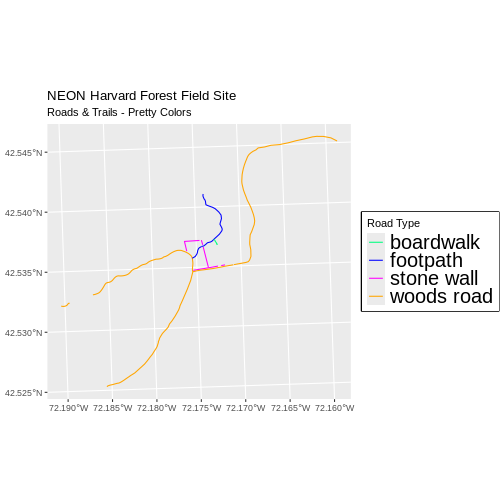
Data Tip
You can modify the default R color palette using the palette method.
For example palette(rainbow(6)) or
palette(terrain.colors(6)). You can reset the palette
colors using palette("default")!
You can also use colorblind-friendly palettes such as those in the viridis package.
Challenge: Plot Lines by Attribute
Create a plot that emphasizes only roads where bicycles and horses
are allowed. To emphasize this, make the lines where bicycles are not
allowed THINNER than the roads where bicycles are allowed. NOTE: this
attribute information is located in the
lines_HARV$BicyclesHo attribute.
Be sure to add a title and legend to your map. You might consider a color palette that has all bike/horse-friendly roads displayed in a bright color. All other lines can be black.
First we explore the BicyclesHo attribute to learn the
values that correspond to the roads we need.
R
lines_HARV %>%
  pull(BicyclesHo) %>%
  unique()
OUTPUT
[1] "Bicycles and Horses Allowed"     NA
[3] "DO NOT SHOW ON REC MAP"          "Bicycles and Horses NOT ALLOWED"
Now, we can create a data frame with only those roads where bicycles and horses are allowed.
R
lines_showHarv <-
  lines_HARV %>%
  filter(BicyclesHo == "Bicycles and Horses Allowed")
Finally, we plot the needed roads after setting them to magenta and a thicker line width.
R
ggplot() +
  geom_sf(data = lines_HARV) +
  geom_sf(data = lines_showHarv, aes(color = BicyclesHo), size = 2) +
  scale_color_manual(values = "magenta") +
  ggtitle("NEON Harvard Forest Field Site",
          subtitle = "Roads Where Bikes and Horses Are Allowed") +
  coord_sf()
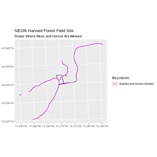
Challenge: Plot Polygon by Attribute
- Create a map of the state boundaries in the United States using the
data located in your downloaded data folder:
NEON-DS-Site-Layout-Files/US-Boundary-Layers\US-State-Boundaries-Census-2014. Apply a line color to each state using itsregionvalue. Add a legend.
First we read in the data and check how many levels there are in the
region column:
R
state_boundary_US <-
st_read("data/NEON-DS-Site-Layout-Files/US-Boundary-Layers/US-State-Boundaries-Census-2014.shp") %>%
# NOTE: We need neither Z nor M coordinates!
st_zm()
OUTPUT
Reading layer `US-State-Boundaries-Census-2014' from data source
  `/home/runner/work/r-raster-vector-geospatial/r-raster-vector-geospatial/site/built/data/NEON-DS-Site-Layout-Files/US-Boundary-Layers/US-State-Boundaries-Census-2014.shp'
  using driver `ESRI Shapefile'
Simple feature collection with 58 features and 10 fields
Geometry type: MULTIPOLYGON
Dimension:     XYZ
Bounding box:  xmin: -124.7258 ymin: 24.49813 xmax: -66.9499 ymax: 49.38436
z_range:       zmin: 0 zmax: 0
Geodetic CRS:  WGS 84
R
state_boundary_US$region <- as.factor(state_boundary_US$region)
levels(state_boundary_US$region)
OUTPUT
[1] "Midwest" "Northeast" "Southeast" "Southwest" "West" Next we set a color vector with that many items:
R
colors <- c("purple", "springgreen", "yellow", "brown", "navy")
Now we can create our plot:
R
ggplot() +
  geom_sf(data = state_boundary_US, aes(color = region), size = 1) +
  scale_color_manual(values = colors) +
  ggtitle("Contiguous U.S. State Boundaries") +
  coord_sf()
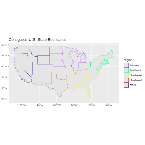
Key Points
- Spatial objects in
sfare similar to standard data frames and can be manipulated using the same functions. - Almost any feature of a plot can be customized using the various
functions and options in the
ggplot2package.
Content from Plot Multiple Vector Layers
Last updated on 2024-10-15 | Edit this page
Overview
Questions
- How can I create map compositions with custom legends using ggplot?
- How can I plot raster and vector data together?
Objectives
- Plot multiple vector layers in the same plot.
- Apply custom symbols to spatial objects in a plot.
- Create a multi-layered plot with raster and vector data.
Things You’ll Need To Complete This Episode
See the lesson homepage for detailed information about the software, data, and other prerequisites you will need to work through the examples in this episode.
This episode builds upon the previous episode to work with vector layers in R and explore how to plot multiple vector layers. It also covers how to plot raster and vector data together on the same plot.
Load the Data
To work with vector data in R, we can use the sf
library. The terra package also allows us to explore
metadata using similar commands for both raster and vector files. Make
sure that you have these packages loaded.
We will continue to work with the three ESRI shapefile
that we loaded in the Open and
Plot Vector Layers in R episode.
Plotting Multiple Vector Layers
In the previous episode, we learned how to plot information from a single vector layer and do some plot customization including adding a custom legend. However, what if we want to create a more complex plot with many vector layers and unique symbols that need to be represented clearly in a legend?
Now, let’s create a plot that combines our tower location
(point_HARV), site boundary
(aoi_boundary_HARV) and roads (lines_HARV)
spatial objects. We will need to build a custom legend as well.
To begin, we will create a plot with the site boundary as the first
layer. Then layer the tower location and road data on top using
+.
R
ggplot() +
  geom_sf(data = aoi_boundary_HARV, fill = "grey", color = "grey") +
  geom_sf(data = lines_HARV, aes(color = TYPE), size = 1) +
  geom_sf(data = point_HARV) +
  ggtitle("NEON Harvard Forest Field Site") +
  coord_sf()
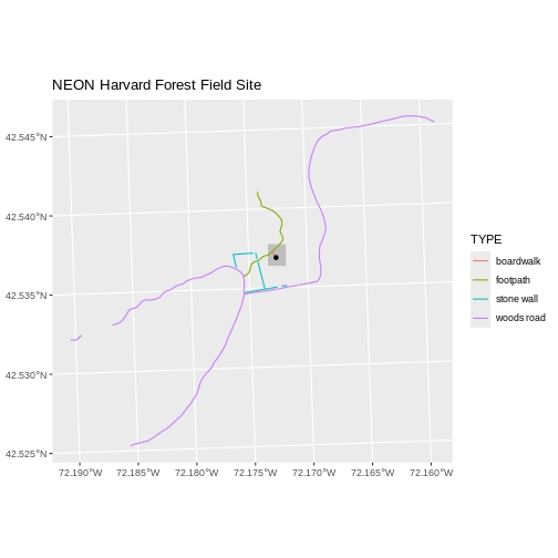
Next, let’s build a custom legend using the symbology (the colors and
symbols) that we used to create the plot above. For example, it might be
good if the lines were symbolized as lines. In the previous episode, you
may have noticed that the default legend behavior for
geom_sf is to draw a ‘patch’ for each legend entry. If you
want the legend to draw lines or points, you need to add an instruction
to the geom_sf call - in this case,
show.legend = 'line'.
R
ggplot() +
  geom_sf(data = aoi_boundary_HARV, fill = "grey", color = "grey") +
  geom_sf(data = lines_HARV, aes(color = TYPE),
          show.legend = "line", size = 1) +
  geom_sf(data = point_HARV, aes(fill = Sub_Type), color = "black") +
  scale_color_manual(values = road_colors) +
  scale_fill_manual(values = "black") +
  ggtitle("NEON Harvard Forest Field Site") +
  coord_sf()
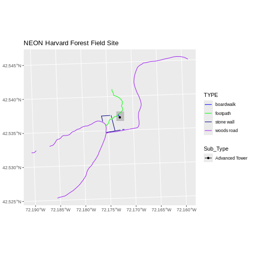
Now lets adjust the legend titles by passing a name to
the respective color and fill palettes.
R
ggplot() +
  geom_sf(data = aoi_boundary_HARV, fill = "grey", color = "grey") +
  geom_sf(data = point_HARV, aes(fill = Sub_Type)) +
  geom_sf(data = lines_HARV, aes(color = TYPE), show.legend = "line",
          size = 1) +
  scale_color_manual(values = road_colors, name = "Line Type") +
  scale_fill_manual(values = "black", name = "Tower Location") +
  ggtitle("NEON Harvard Forest Field Site") +
  coord_sf()

Finally, it might be better if the points were symbolized as a
symbol. We can customize this using shape parameters in our
call to geom_sf: 16 is a point symbol, 15 is a box.
Data Tip
To view a short list of shape symbols, type
?pch into the R console.
R
ggplot() +
  geom_sf(data = aoi_boundary_HARV, fill = "grey", color = "grey") +
  geom_sf(data = point_HARV, aes(fill = Sub_Type), shape = 15) +
  geom_sf(data = lines_HARV, aes(color = TYPE),
          show.legend = "line", size = 1) +
  scale_color_manual(values = road_colors, name = "Line Type") +
  scale_fill_manual(values = "black", name = "Tower Location") +
  ggtitle("NEON Harvard Forest Field Site") +
  coord_sf()
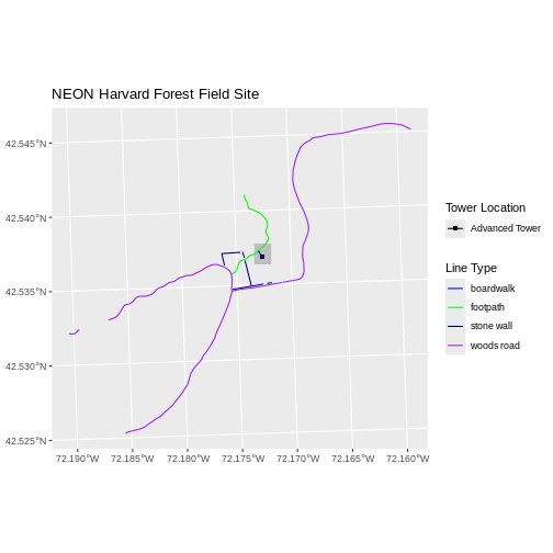
Challenge: Plot Polygon by Attribute
Using the
NEON-DS-Site-Layout-Files/HARV/PlotLocations_HARV.shpESRIshapefile, create a map of study plot locations, with each point colored by the soil type (soilTypeOr). How many different soil types are there at this particular field site? Overlay this layer on top of thelines_HARVlayer (the roads). Create a custom legend that applies line symbols to lines and point symbols to the points.Modify the plot above. Tell R to plot each point, using a different symbol of
shapevalue.
First we need to read in the data and see how many unique soils are
represented in the soilTypeOr attribute.
R
plot_locations <-
  st_read("data/NEON-DS-Site-Layout-Files/HARV/PlotLocations_HARV.shp")
OUTPUT
Reading layer `PlotLocations_HARV' from data source
  `/home/runner/work/r-raster-vector-geospatial/r-raster-vector-geospatial/site/built/data/NEON-DS-Site-Layout-Files/HARV/PlotLocations_HARV.shp'
  using driver `ESRI Shapefile'
Simple feature collection with 21 features and 25 fields
Geometry type: POINT
Dimension:     XY
Bounding box:  xmin: 731405.3 ymin: 4712845 xmax: 732275.3 ymax: 4713846
Projected CRS: WGS 84 / UTM zone 18N
R
plot_locations$soilTypeOr <- as.factor(plot_locations$soilTypeOr)
levels(plot_locations$soilTypeOr)
OUTPUT
[1] "Histosols" "Inceptisols"Next we can create a new color palette with one color for each soil type.
R
blue_orange <- c("cornflowerblue", "darkorange")
Finally, we will create our plot.
R
ggplot() +
  geom_sf(data = lines_HARV, aes(color = TYPE), show.legend = "line") +
  geom_sf(data = plot_locations, aes(fill = soilTypeOr),
          shape = 21, show.legend = 'point') +
  scale_color_manual(name = "Line Type", values = road_colors,
     guide = guide_legend(override.aes = list(linetype = "solid",
                                              shape = NA))) +
  scale_fill_manual(name = "Soil Type", values = blue_orange,
     guide = guide_legend(override.aes = list(linetype = "blank", shape = 21,
                                              colour = NA))) +
  ggtitle("NEON Harvard Forest Field Site") +
  coord_sf()
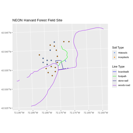
If we want each soil to be shown with a different symbol, we can give
multiple values to the scale_shape_manual() argument.
R
ggplot() +
  geom_sf(data = lines_HARV, aes(color = TYPE), show.legend = "line", size = 1) +
  geom_sf(data = plot_locations, aes(fill = soilTypeOr, shape = soilTypeOr),
          show.legend = 'point', size = 3) +
  scale_shape_manual(name = "Soil Type", values = c(21, 22)) +
  scale_color_manual(name = "Line Type", values = road_colors,
     guide = guide_legend(override.aes = list(linetype = "solid", shape = NA))) +
  scale_fill_manual(name = "Soil Type", values = blue_orange,
     guide = guide_legend(override.aes = list(linetype = "blank", shape = c(21, 22),
     color = blue_orange))) +
  ggtitle("NEON Harvard Forest Field Site") +
  coord_sf()
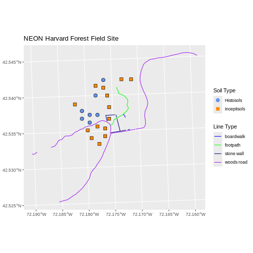
Challenge: Plot Raster & Vector Data Together
You can plot vector data layered on top of raster data using the
+ to add a layer in ggplot. Create a plot that
uses the NEON AOI Canopy Height Model
data/NEON-DS-Airborne-Remote-Sensing/HARV/CHM/HARV_chmCrop.tif
as a base layer. On top of the CHM, please add:
- The study site AOI.
- Roads.
- The tower location.
Be sure to give your plot a meaningful title.
R
ggplot() +
  geom_raster(data = CHM_HARV_df, aes(x = x, y = y, fill = HARV_chmCrop)) +
  geom_sf(data = lines_HARV, color = "black") +
  geom_sf(data = aoi_boundary_HARV, color = "grey20", size = 1) +
  geom_sf(data = point_HARV, pch = 8) +
  ggtitle("NEON Harvard Forest Field Site w/ Canopy Height Model") +
  coord_sf()
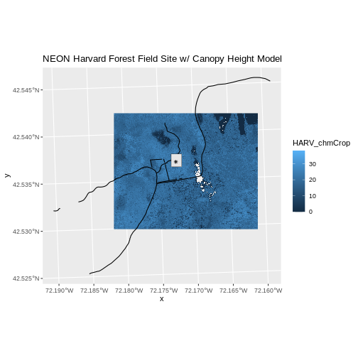
Key Points
- Use the
+operator to add multiple layers to a ggplot. - Multi-layered plots can combine raster and vector datasets.
- Use the
show.legendargument to set legend symbol types. - Use the
scale_fill_manual()function to set legend colors.
Content from Handling Spatial Projection & CRS
Last updated on 2024-10-15 | Edit this page
Overview
Questions
- What do I do when vector data don’t line up?
Objectives
- Plot vector objects with different CRSs in the same plot.
Things You’ll Need To Complete This Episode
See the lesson homepage for detailed information about the software, data, and other prerequisites you will need to work through the examples in this episode.
In an earlier episode we learned how to handle a situation where you have two different files with raster data in different projections. Now we will apply those same principles to working with vector data. We will create a base map of our study site using United States state and country boundary information accessed from the United States Census Bureau. We will learn how to map vector data that are in different CRSs and thus don’t line up on a map.
We will continue to work with the three ESRI shapefiles
that we loaded in the Open and
Plot Vector Layers in R episode.
Working With Spatial Data From Different Sources
We often need to gather spatial datasets from different sources and/or data that cover different spatial extents. These data are often in different Coordinate Reference Systems (CRSs).
Some reasons for data being in different CRSs include:
- The data are stored in a particular CRS convention used by the data provider (for example, a government agency).
- The data are stored in a particular CRS that is customized to a region. For instance, many states in the US prefer to use a State Plane projection customized for that state.
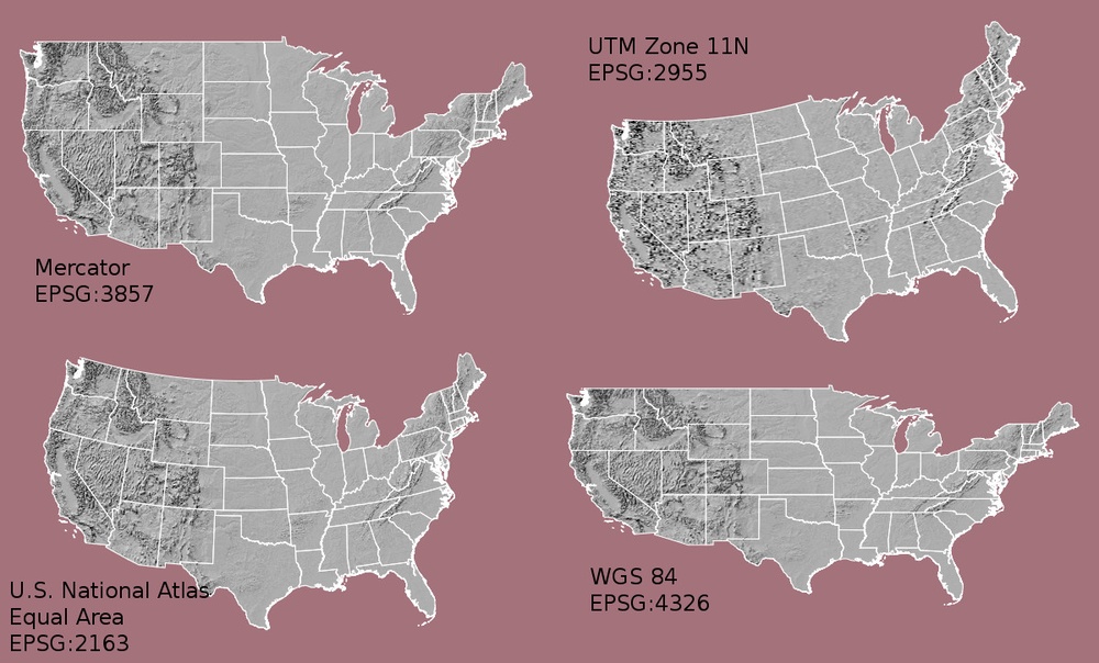 {alt=’Maps
of the United States using data in different projections.}
{alt=’Maps
of the United States using data in different projections.}
Notice the differences in shape associated with each different projection. These differences are a direct result of the calculations used to “flatten” the data onto a 2-dimensional map. Often data are stored purposefully in a particular projection that optimizes the relative shape and size of surrounding geographic boundaries (states, counties, countries, etc).
In this episode we will learn how to identify and manage spatial data in different projections. We will learn how to reproject the data so that they are in the same projection to support plotting / mapping. Note that these skills are also required for any geoprocessing / spatial analysis. Data need to be in the same CRS to ensure accurate results.
We will continue to use the sf and terra
packages in this episode.
Import US Boundaries - Census Data
There are many good sources of boundary base layers that we can use
to create a basemap. Some R packages even have these base layers built
in to support quick and efficient mapping. In this episode, we will use
boundary layers for the contiguous United States, provided by the United
States Census Bureau. It is useful to have vector layers in ESRI’s
shapefile format to work with because we can add additional
attributes to them if need be - for project specific mapping.
Read US Boundary File
We will use the st_read() function to import the
/US-Boundary-Layers/US-State-Boundaries-Census-2014 layer
into R. This layer contains the boundaries of all contiguous states in
the U.S. Please note that these data have been modified and reprojected
from the original data downloaded from the Census website to support the
learning goals of this episode.
R
state_boundary_US <- st_read("data/NEON-DS-Site-Layout-Files/US-Boundary-Layers/US-State-Boundaries-Census-2014.shp") %>%
  st_zm()
OUTPUT
Reading layer `US-State-Boundaries-Census-2014' from data source
  `/home/runner/work/r-raster-vector-geospatial/r-raster-vector-geospatial/site/built/data/NEON-DS-Site-Layout-Files/US-Boundary-Layers/US-State-Boundaries-Census-2014.shp'
  using driver `ESRI Shapefile'
Simple feature collection with 58 features and 10 fields
Geometry type: MULTIPOLYGON
Dimension:     XYZ
Bounding box:  xmin: -124.7258 ymin: 24.49813 xmax: -66.9499 ymax: 49.38436
z_range:       zmin: 0 zmax: 0
Geodetic CRS:  WGS 84
Next, let’s plot the U.S. states data:
R
ggplot() +
  geom_sf(data = state_boundary_US) +
  ggtitle("Map of Contiguous US State Boundaries") +
  coord_sf()
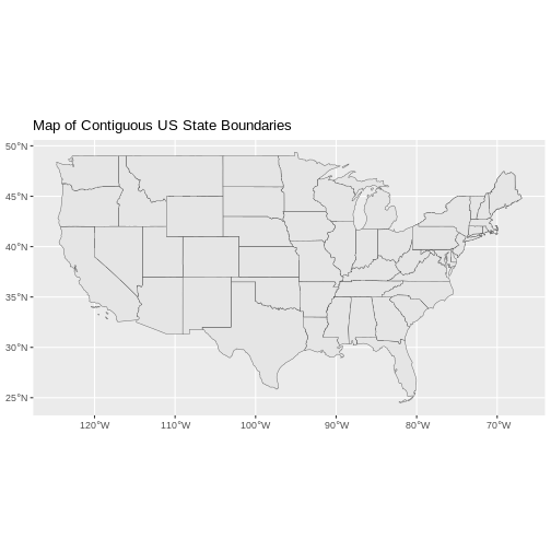
U.S. Boundary Layer
We can add a boundary layer of the United States to our map - to make
it look nicer. We will import
NEON-DS-Site-Layout-Files/US-Boundary-Layers/US-Boundary-Dissolved-States.
R
country_boundary_US <- st_read("data/NEON-DS-Site-Layout-Files/US-Boundary-Layers/US-Boundary-Dissolved-States.shp") %>%
  st_zm()
OUTPUT
Reading layer `US-Boundary-Dissolved-States' from data source
  `/home/runner/work/r-raster-vector-geospatial/r-raster-vector-geospatial/site/built/data/NEON-DS-Site-Layout-Files/US-Boundary-Layers/US-Boundary-Dissolved-States.shp'
  using driver `ESRI Shapefile'
Simple feature collection with 1 feature and 9 fields
Geometry type: MULTIPOLYGON
Dimension:     XYZ
Bounding box:  xmin: -124.7258 ymin: 24.49813 xmax: -66.9499 ymax: 49.38436
z_range:       zmin: 0 zmax: 0
Geodetic CRS:  WGS 84
If we specify a thicker line width using size = 2 for
the border layer, it will make our map pop! We will also manually set
the colors of the state boundaries and country boundaries.
R
ggplot() +
  geom_sf(data = state_boundary_US, color = "gray60") +
  geom_sf(data = country_boundary_US, color = "black",alpha = 0.25,size = 5) +
  ggtitle("Map of Contiguous US State Boundaries") +
  coord_sf()
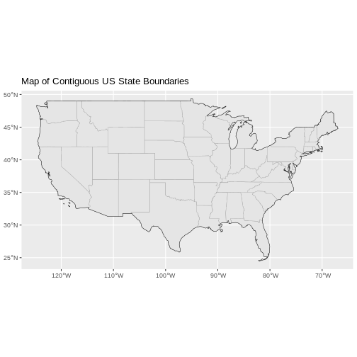
Next, let’s add the location of a flux tower where our study area is. As we are adding these layers, take note of the CRS of each object. First let’s look at the CRS of our tower location object:
R
st_crs(point_HARV)$proj4string
OUTPUT
[1] "+proj=utm +zone=18 +datum=WGS84 +units=m +no_defs"Our project string for point_HARV specifies the UTM
projection as follows:
+proj=utm +zone=18 +datum=WGS84 +units=m +no_defs
- proj=utm: the projection is UTM, UTM has several zones.
- zone=18: the zone is 18
- datum=WGS84: the datum WGS84 (the datum refers to the 0,0 reference for the coordinate system used in the projection)
- units=m: the units for the coordinates are in METERS.
Note that the zone is unique to the UTM projection. Not
all CRSs will have a zone.
Let’s check the CRS of our state and country boundary objects:
R
st_crs(state_boundary_US)$proj4string
OUTPUT
[1] "+proj=longlat +datum=WGS84 +no_defs"R
st_crs(country_boundary_US)$proj4string
OUTPUT
[1] "+proj=longlat +datum=WGS84 +no_defs"Our project string for state_boundary_US and
country_boundary_US specifies the lat/long projection as
follows:
+proj=longlat +datum=WGS84 +no_defs
- proj=longlat: the data are in a geographic (latitude and longitude) coordinate system
- datum=WGS84: the datum WGS84 (the datum refers to the 0,0 reference for the coordinate system used in the projection)
- no_defs: ensures that no defaults are used, but this is now obsolete
Note that there are no specified units above. This is because this geographic coordinate reference system is in latitude and longitude which is most often recorded in decimal degrees.
Data Tip
the last portion of each proj4 string could potentially
be something like +towgs84=0,0,0. This is a conversion
factor that is used if a datum conversion is required. We will not deal
with datums in this episode series.
CRS Units - View Object Extent
Next, let’s view the extent or spatial coverage for the
point_HARV spatial object compared to the
state_boundary_US object.
First we’ll look at the extent for our study site:
R
st_bbox(point_HARV)
OUTPUT
     xmin      ymin      xmax      ymax
 732183.2 4713265.0  732183.2 4713265.0
And then the extent for the state boundary data.
R
st_bbox(state_boundary_US)
OUTPUT
      xmin       ymin       xmax       ymax
-124.72584   24.49813  -66.94989   49.38436
Note the difference in the units for each object. The extent for
state_boundary_US is in latitude and longitude which yields
smaller numbers representing decimal degree units. Our tower location
point is in UTM, is represented in meters.
Proj4 & CRS Resources
- Official PROJ library documentation
- More information on the proj4 format.
- A fairly comprehensive list of CRSs by format.
- To view a list of datum conversion factors type:
sf_proj_info(type = "datum")into the R console. However, the results would depend on the underlying version of the PROJ library.
Reproject Vector Data or No?
We saw in an earlier episode
that when working with raster data in different CRSs, we needed to
convert all objects to the same CRS. We can do the same thing with our
vector data - however, we don’t need to! When using the
ggplot2 package, ggplot automatically converts
all objects to the same CRS before plotting. This means we can plot our
three data sets together without doing any conversion:
R
ggplot() +
  geom_sf(data = state_boundary_US, color = "gray60") +
  geom_sf(data = country_boundary_US, size = 5, alpha = 0.25, color = "black") +
  geom_sf(data = point_HARV, shape = 19, color = "purple") +
  ggtitle("Map of Contiguous US State Boundaries") +
  coord_sf()
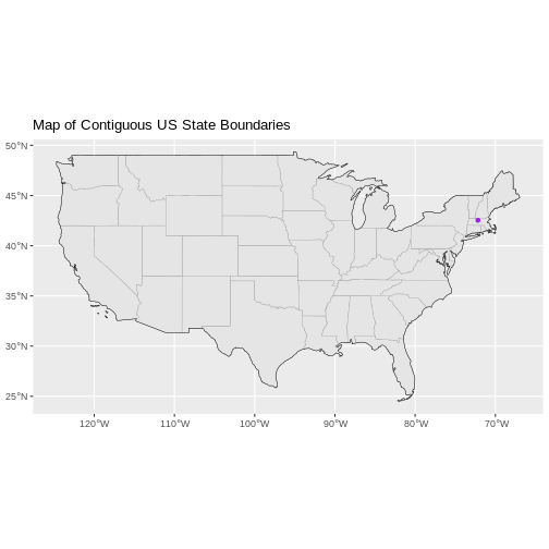
Challenge - Plot Multiple Layers of Spatial Data
Create a map of the North Eastern United States as follows:
- Import and plot
Boundary-US-State-NEast.shp. Adjust line width as necessary. - Layer the Fisher Tower (in the NEON Harvard Forest site) point
location
point_HARVonto the plot. - Add a title.
- Add a legend that shows both the state boundary (as a line) and the Tower location point.
R
NE.States.Boundary.US <- st_read("data/NEON-DS-Site-Layout-Files/US-Boundary-Layers/Boundary-US-State-NEast.shp") %>%
  st_zm()
OUTPUT
Reading layer `Boundary-US-State-NEast' from data source
  `/home/runner/work/r-raster-vector-geospatial/r-raster-vector-geospatial/site/built/data/NEON-DS-Site-Layout-Files/US-Boundary-Layers/Boundary-US-State-NEast.shp'
  using driver `ESRI Shapefile'
Simple feature collection with 12 features and 9 fields
Geometry type: MULTIPOLYGON
Dimension:     XYZ
Bounding box:  xmin: -80.51989 ymin: 37.91685 xmax: -66.9499 ymax: 47.45716
z_range:       zmin: 0 zmax: 0
Geodetic CRS:  WGS 84
R
ggplot() +
    geom_sf(data = NE.States.Boundary.US, aes(color ="color"),
            show.legend = "line") +
    scale_color_manual(name = "", labels = "State Boundary",
                       values = c("color" = "gray18")) +
    geom_sf(data = point_HARV, aes(shape = "shape"), color = "purple") +
    scale_shape_manual(name = "", labels = "Fisher Tower",
                       values = c("shape" = 19)) +
    ggtitle("Fisher Tower location") +
    theme(legend.background = element_rect(color = NA)) +
    coord_sf()
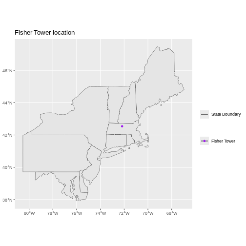
Key Points
-
ggplot2automatically converts all objects in a plot to the same CRS. - Still be aware of the CRS and extent for each object.
Content from Convert from .csv to a Vector Layer
Last updated on 2024-10-15 | Edit this page
Overview
Questions
- How can I import CSV files as vector layers in R?
Objectives
- Import .csv files containing x,y coordinate locations into R as a data frame.
- Convert a data frame to a spatial object.
- Export a spatial object to a text file.
Things You’ll Need To Complete This Episode
See the lesson homepage for detailed information about the software, data, and other prerequisites you will need to work through the examples in this episode.
This episode will review how to import spatial points stored in
.csv (Comma Separated Value) format into R as an
sf spatial object. We will also reproject data imported
from an ESRI shapefile format, export the reprojected data
as an ESRI shapefile, and plot raster and vector data as
layers in the same plot.
Spatial Data in Text Format
The HARV_PlotLocations.csv file contains
x, y (point) locations for study plot where NEON collects
data on vegetation
and other ecological metics. We would like to:
- Create a map of these plot locations.
- Export the data in an ESRI
shapefileformat to share with our colleagues. Thisshapefilecan be imported into most GIS software. - Create a map showing vegetation height with plot locations layered on top.
Spatial data are sometimes stored in a text file format
(.txt or .csv). If the text file has an
associated x and y location column, then we
can convert it into an sf spatial object. The
sf object allows us to store both the x,y
values that represent the coordinate location of each point and the
associated attribute data - or columns describing each feature in the
spatial object.
We will continue using the sf and terra
packages in this episode.
Import .csv
To begin let’s import a .csv file that contains plot
coordinate x, y locations at the NEON Harvard Forest Field
Site (HARV_PlotLocations.csv) and look at the structure of
that new object:
R
plot_locations_HARV <-
  read.csv("data/NEON-DS-Site-Layout-Files/HARV/HARV_PlotLocations.csv")

str(plot_locations_HARV)
OUTPUT
'data.frame':	21 obs. of  16 variables:
 $ easting   : num  731405 731934 731754 731724 732125 ...
 $ northing  : num  4713456 4713415 4713115 4713595 4713846 ...
 $ geodeticDa: chr  "WGS84" "WGS84" "WGS84" "WGS84" ...
 $ utmZone   : chr  "18N" "18N" "18N" "18N" ...
 $ plotID    : chr  "HARV_015" "HARV_033" "HARV_034" "HARV_035" ...
 $ stateProvi: chr  "MA" "MA" "MA" "MA" ...
 $ county    : chr  "Worcester" "Worcester" "Worcester" "Worcester" ...
 $ domainName: chr  "Northeast" "Northeast" "Northeast" "Northeast" ...
 $ domainID  : chr  "D01" "D01" "D01" "D01" ...
 $ siteID    : chr  "HARV" "HARV" "HARV" "HARV" ...
 $ plotType  : chr  "distributed" "tower" "tower" "tower" ...
 $ subtype   : chr  "basePlot" "basePlot" "basePlot" "basePlot" ...
 $ plotSize  : int  1600 1600 1600 1600 1600 1600 1600 1600 1600 1600 ...
 $ elevation : num  332 342 348 334 353 ...
 $ soilTypeOr: chr  "Inceptisols" "Inceptisols" "Inceptisols" "Histosols" ...
 $ plotdim_m : int  40 40 40 40 40 40 40 40 40 40 ...
We now have a data frame that contains 21 locations (rows) and 16
variables (attributes). Note that all of our character data was imported
into R as character (text) data. Next, let’s explore the dataframe to
determine whether it contains columns with coordinate values. If we are
lucky, our .csv will contain columns labeled:
- “X” and “Y” OR
- Latitude and Longitude OR
- easting and northing (UTM coordinates)
Let’s check out the column names of our dataframe.
R
names(plot_locations_HARV)
OUTPUT
 [1] "easting"    "northing"   "geodeticDa" "utmZone"    "plotID"
 [6] "stateProvi" "county"     "domainName" "domainID"   "siteID"
[11] "plotType"   "subtype"    "plotSize"   "elevation"  "soilTypeOr"
[16] "plotdim_m"
Identify X,Y Location Columns
Our column names include several fields that might contain spatial
information. The plot_locations_HARV$easting and
plot_locations_HARV$northing columns contain coordinate
values. We can confirm this by looking at the first six rows of our
data.
R
head(plot_locations_HARV$easting)
OUTPUT
[1] 731405.3 731934.3 731754.3 731724.3 732125.3 731634.3R
head(plot_locations_HARV$northing)
OUTPUT
[1] 4713456 4713415 4713115 4713595 4713846 4713295We have coordinate values in our data frame. In order to convert our
data frame to an sf object, we also need to know the CRS
associated with those coordinate values.
There are several ways to figure out the CRS of spatial data in text format.
- We can check the file metadata in hopes that the CRS was recorded in the data.
- We can explore the file itself to see if CRS information is embedded in the file header or somewhere in the data columns.
Following the easting and northing columns,
there is a geodeticDa and a utmZone column.
These appear to contain CRS information (datum and
projection). Let’s view those next.
R
head(plot_locations_HARV$geodeticDa)
OUTPUT
[1] "WGS84" "WGS84" "WGS84" "WGS84" "WGS84" "WGS84"R
head(plot_locations_HARV$utmZone)
OUTPUT
[1] "18N" "18N" "18N" "18N" "18N" "18N"It is not typical to store CRS information in a column. But this
particular file contains CRS information this way. The
geodeticDa and utmZone columns contain the
information that helps us determine the CRS:
-
geodeticDa: WGS84 – this is geodetic datum WGS84 -
utmZone: 18
In When Vector
Data Don’t Line Up - Handling Spatial Projection & CRS in R we
learned about the components of a proj4 string. We have
everything we need to assign a CRS to our data frame.
To create the proj4 associated with UTM Zone 18 WGS84 we
can look up the projection on the Spatial Reference
website, which contains a list of CRS formats for each projection.
From here, we can extract the proj4
string for UTM Zone 18N WGS84.
However, if we have other data in the UTM Zone 18N projection, it’s
much easier to use the st_crs() function to extract the CRS
in proj4 format from that object and assign it to our new
spatial object. We’ve seen this CRS before with our Harvard Forest study
site (point_HARV).
R
st_crs(point_HARV)
OUTPUT
Coordinate Reference System:
  User input: WGS 84 / UTM zone 18N
  wkt:
PROJCRS["WGS 84 / UTM zone 18N",
    BASEGEOGCRS["WGS 84",
        DATUM["World Geodetic System 1984",
            ELLIPSOID["WGS 84",6378137,298.257223563,
                LENGTHUNIT["metre",1]]],
        PRIMEM["Greenwich",0,
            ANGLEUNIT["degree",0.0174532925199433]],
        ID["EPSG",4326]],
    CONVERSION["UTM zone 18N",
        METHOD["Transverse Mercator",
            ID["EPSG",9807]],
        PARAMETER["Latitude of natural origin",0,
            ANGLEUNIT["Degree",0.0174532925199433],
            ID["EPSG",8801]],
        PARAMETER["Longitude of natural origin",-75,
            ANGLEUNIT["Degree",0.0174532925199433],
            ID["EPSG",8802]],
        PARAMETER["Scale factor at natural origin",0.9996,
            SCALEUNIT["unity",1],
            ID["EPSG",8805]],
        PARAMETER["False easting",500000,
            LENGTHUNIT["metre",1],
            ID["EPSG",8806]],
        PARAMETER["False northing",0,
            LENGTHUNIT["metre",1],
            ID["EPSG",8807]]],
    CS[Cartesian,2],
        AXIS["(E)",east,
            ORDER[1],
            LENGTHUNIT["metre",1]],
        AXIS["(N)",north,
            ORDER[2],
            LENGTHUNIT["metre",1]],
    ID["EPSG",32618]]
The output above shows that the points vector layer is in UTM zone
18N. We can thus use the CRS from that spatial object to convert our
non-spatial dataframe into an sf object.
Next, let’s create a crs object that we can use to
define the CRS of our sf object when we create it.
R
utm18nCRS <- st_crs(point_HARV)
utm18nCRS
OUTPUT
Coordinate Reference System:
  User input: WGS 84 / UTM zone 18N
  wkt:
PROJCRS["WGS 84 / UTM zone 18N",
    BASEGEOGCRS["WGS 84",
        DATUM["World Geodetic System 1984",
            ELLIPSOID["WGS 84",6378137,298.257223563,
                LENGTHUNIT["metre",1]]],
        PRIMEM["Greenwich",0,
            ANGLEUNIT["degree",0.0174532925199433]],
        ID["EPSG",4326]],
    CONVERSION["UTM zone 18N",
        METHOD["Transverse Mercator",
            ID["EPSG",9807]],
        PARAMETER["Latitude of natural origin",0,
            ANGLEUNIT["Degree",0.0174532925199433],
            ID["EPSG",8801]],
        PARAMETER["Longitude of natural origin",-75,
            ANGLEUNIT["Degree",0.0174532925199433],
            ID["EPSG",8802]],
        PARAMETER["Scale factor at natural origin",0.9996,
            SCALEUNIT["unity",1],
            ID["EPSG",8805]],
        PARAMETER["False easting",500000,
            LENGTHUNIT["metre",1],
            ID["EPSG",8806]],
        PARAMETER["False northing",0,
            LENGTHUNIT["metre",1],
            ID["EPSG",8807]]],
    CS[Cartesian,2],
        AXIS["(E)",east,
            ORDER[1],
            LENGTHUNIT["metre",1]],
        AXIS["(N)",north,
            ORDER[2],
            LENGTHUNIT["metre",1]],
    ID["EPSG",32618]]
R
class(utm18nCRS)
OUTPUT
[1] "crs".csv to sf object
Next, let’s convert our dataframe into an sf object. To
do this, we need to specify:
- The columns containing X (
easting) and Y (northing) coordinate values - The CRS that the column coordinate represent (units are included in
the CRS) - stored in our
utmCRSobject.
We will use the st_as_sf() function to perform the
conversion.
R
plot_locations_sp_HARV <- st_as_sf(plot_locations_HARV,
                                   coords = c("easting", "northing"),
                                   crs = utm18nCRS)
We should double check the CRS to make sure it is correct.
R
st_crs(plot_locations_sp_HARV)
OUTPUT
Coordinate Reference System:
  User input: WGS 84 / UTM zone 18N
  wkt:
PROJCRS["WGS 84 / UTM zone 18N",
    BASEGEOGCRS["WGS 84",
        DATUM["World Geodetic System 1984",
            ELLIPSOID["WGS 84",6378137,298.257223563,
                LENGTHUNIT["metre",1]]],
        PRIMEM["Greenwich",0,
            ANGLEUNIT["degree",0.0174532925199433]],
        ID["EPSG",4326]],
    CONVERSION["UTM zone 18N",
        METHOD["Transverse Mercator",
            ID["EPSG",9807]],
        PARAMETER["Latitude of natural origin",0,
            ANGLEUNIT["Degree",0.0174532925199433],
            ID["EPSG",8801]],
        PARAMETER["Longitude of natural origin",-75,
            ANGLEUNIT["Degree",0.0174532925199433],
            ID["EPSG",8802]],
        PARAMETER["Scale factor at natural origin",0.9996,
            SCALEUNIT["unity",1],
            ID["EPSG",8805]],
        PARAMETER["False easting",500000,
            LENGTHUNIT["metre",1],
            ID["EPSG",8806]],
        PARAMETER["False northing",0,
            LENGTHUNIT["metre",1],
            ID["EPSG",8807]]],
    CS[Cartesian,2],
        AXIS["(E)",east,
            ORDER[1],
            LENGTHUNIT["metre",1]],
        AXIS["(N)",north,
            ORDER[2],
            LENGTHUNIT["metre",1]],
    ID["EPSG",32618]]
Plot Spatial Object
We now have a spatial R object, we can plot our newly created spatial object.
R
ggplot() +
  geom_sf(data = plot_locations_sp_HARV) +
  ggtitle("Map of Plot Locations")
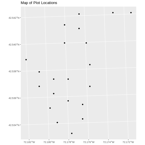
Plot Extent
In Open and Plot Vector
Layers in R we learned about spatial object extent. When we plot
several spatial layers in R using ggplot, all of the layers
of the plot are considered in setting the boundaries of the plot. To
show this, let’s plot our aoi_boundary_HARV object with our
vegetation plots.
R
ggplot() +
  geom_sf(data = aoi_boundary_HARV) +
  geom_sf(data = plot_locations_sp_HARV) +
  ggtitle("AOI Boundary Plot")
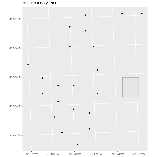
When we plot the two layers together, ggplot sets the
plot boundaries so that they are large enough to include all of the data
included in all of the layers. That’s really handy!
Challenge - Import & Plot Additional Points
We want to add two phenology plots to our existing map of vegetation plot locations.
Import the .csv: HARV/HARV_2NewPhenPlots.csv into R and
do the following:
- Find the X and Y coordinate locations. Which value is X and which value is Y?
- These data were collected in a geographic coordinate system (WGS84).
Convert the dataframe into an
sfobject. - Plot the new points with the plot location points from above. Be sure to add a legend. Use a different symbol for the 2 new points!
If you have extra time, feel free to add roads and other layers to your map!
- First we will read in the new csv file and look at the data structure.
R
newplot_locations_HARV <-
  read.csv("data/NEON-DS-Site-Layout-Files/HARV/HARV_2NewPhenPlots.csv")
str(newplot_locations_HARV)
OUTPUT
'data.frame':	2 obs. of  13 variables:
 $ decimalLat: num  42.5 42.5
 $ decimalLon: num  -72.2 -72.2
 $ country   : chr  "unitedStates" "unitedStates"
 $ stateProvi: chr  "MA" "MA"
 $ county    : chr  "Worcester" "Worcester"
 $ domainName: chr  "Northeast" "Northeast"
 $ domainID  : chr  "D01" "D01"
 $ siteID    : chr  "HARV" "HARV"
 $ plotType  : chr  "tower" "tower"
 $ subtype   : chr  "phenology" "phenology"
 $ plotSize  : int  40000 40000
 $ plotDimens: chr  "200m x 200m" "200m x 200m"
$ elevation : num 358 346- The US boundary data we worked with previously is in a geographic
WGS84 CRS. We can use that data to establish a CRS for this data. First
we will extract the CRS from the
country_boundary_USobject and confirm that it is WGS84.
R
geogCRS <- st_crs(country_boundary_US)
geogCRS
OUTPUT
Coordinate Reference System:
  User input: WGS 84
  wkt:
GEOGCRS["WGS 84",
    DATUM["World Geodetic System 1984",
        ELLIPSOID["WGS 84",6378137,298.257223563,
            LENGTHUNIT["metre",1]]],
    PRIMEM["Greenwich",0,
        ANGLEUNIT["degree",0.0174532925199433]],
    CS[ellipsoidal,2],
        AXIS["latitude",north,
            ORDER[1],
            ANGLEUNIT["degree",0.0174532925199433]],
        AXIS["longitude",east,
            ORDER[2],
            ANGLEUNIT["degree",0.0174532925199433]],
    ID["EPSG",4326]]
Then we will convert our new data to a spatial dataframe, using the
geogCRS object as our CRS.
R
newPlot.Sp.HARV <- st_as_sf(newplot_locations_HARV,
                            coords = c("decimalLon", "decimalLat"),
                            crs = geogCRS)
Next we’ll confirm that the CRS for our new object is correct.
R
st_crs(newPlot.Sp.HARV)
OUTPUT
Coordinate Reference System:
  User input: WGS 84
  wkt:
GEOGCRS["WGS 84",
    DATUM["World Geodetic System 1984",
        ELLIPSOID["WGS 84",6378137,298.257223563,
            LENGTHUNIT["metre",1]]],
    PRIMEM["Greenwich",0,
        ANGLEUNIT["degree",0.0174532925199433]],
    CS[ellipsoidal,2],
        AXIS["latitude",north,
            ORDER[1],
            ANGLEUNIT["degree",0.0174532925199433]],
        AXIS["longitude",east,
            ORDER[2],
            ANGLEUNIT["degree",0.0174532925199433]],
    ID["EPSG",4326]]
We will be adding these new data points to the plot we created
before. The data for the earlier plot was in UTM. Since we’re using
ggplot, it will reproject the data for us.
- Now we can create our plot.
R
ggplot() +
  geom_sf(data = plot_locations_sp_HARV, color = "orange") +
  geom_sf(data = newPlot.Sp.HARV, color = "lightblue") +
  ggtitle("Map of All Plot Locations")
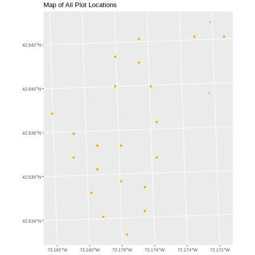
Export to an ESRI shapefile
We can write an R spatial object to an ESRI shapefile
using the st_write function in sf. To do this
we need the following arguments:
- the name of the spatial object
(
plot_locations_sp_HARV) - the directory where we want to save our ESRI
shapefile(to usecurrent = getwd()or you can specify a different path) - the name of the new ESRI
shapefile(PlotLocations_HARV) - the driver which specifies the file format (ESRI Shapefile)
We can now export the spatial object as an ESRI
shapefile.
R
st_write(plot_locations_sp_HARV,
         "data/PlotLocations_HARV.shp", driver = "ESRI Shapefile")
Key Points
- Know the projection (if any) of your point data prior to converting to a spatial object.
- Convert a data frame to an
sfobject using thest_as_sf()function. - Export an
sfobject as text using thest_write()function.
Content from Manipulate Raster Data
Last updated on 2024-10-15 | Edit this page
Overview
Questions
- How can I crop raster objects to vector objects, and extract the summary of raster pixels?
Objectives
- Crop a raster to the extent of a vector layer.
- Extract values from a raster that correspond to a vector file overlay.
Things You’ll Need To Complete This Episode
See the lesson homepage for detailed information about the software, data, and other prerequisites you will need to work through the examples in this episode.
This episode explains how to crop a raster using the extent of a vector layer. We will also cover how to extract values from a raster that occur within a set of polygons, or in a buffer (surrounding) region around a set of points.
Crop a Raster to Vector Extent
We often work with spatial layers that have different spatial extents. The spatial extent of a vector layer or R spatial object represents the geographic “edge” or location that is the furthest north, south east and west. Thus it represents the overall geographic coverage of the spatial object.
Image Source: National Ecological
Observatory Network (NEON)
The graphic below illustrates the extent of several of the spatial layers that we have worked with in this workshop:
- Area of interest (AOI) – blue
- Roads and trails – purple
- Vegetation plot locations (marked with white dots)– black
- A canopy height model (CHM) in GeoTIFF format – green

Frequent use cases of cropping a raster file include reducing file size and creating maps. Sometimes we have a raster file that is much larger than our study area or area of interest. It is often more efficient to crop the raster to the extent of our study area to reduce file sizes as we process our data. Cropping a raster can also be useful when creating pretty maps so that the raster layer matches the extent of the desired vector layers.
Crop a Raster Using Vector Extent
We can use the crop() function to crop a raster to the
extent of another spatial object. To do this, we need to specify the
raster to be cropped and the spatial object that will be used to crop
the raster. R will use the extent of the spatial object as
the cropping boundary.
To illustrate this, we will crop the Canopy Height Model (CHM) to
only include the area of interest (AOI). Let’s start by plotting the
full extent of the CHM data and overlay where the AOI falls within it.
The boundaries of the AOI will be colored blue, and we use
fill = NA to make the area transparent.
R
ggplot() +
  geom_raster(data = CHM_HARV_df, aes(x = x, y = y, fill = HARV_chmCrop)) +
  scale_fill_gradientn(name = "Canopy Height", colors = terrain.colors(10)) +
  geom_sf(data = aoi_boundary_HARV, color = "blue", fill = NA) +
  coord_sf()
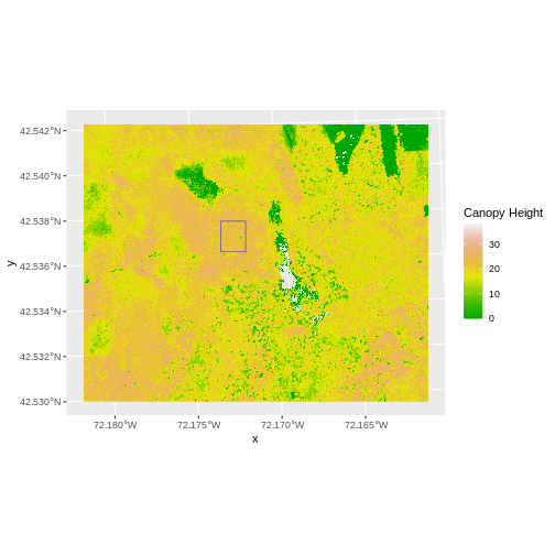
Now that we have visualized the area of the CHM we want to subset, we
can perform the cropping operation. We are going to crop()
function from the raster package to create a new object with only the
portion of the CHM data that falls within the boundaries of the AOI.
R
CHM_HARV_Cropped <- crop(x = CHM_HARV, y = aoi_boundary_HARV)
Now we can plot the cropped CHM data, along with a boundary box
showing the full CHM extent. However, remember, since this is raster
data, we need to convert to a data frame in order to plot using
ggplot. To get the boundary box from CHM, the
st_bbox() will extract the 4 corners of the rectangle that
encompass all the features contained in this object. The
st_as_sfc() converts these 4 coordinates into a polygon
that we can plot:
R
CHM_HARV_Cropped_df <- as.data.frame(CHM_HARV_Cropped, xy = TRUE)

ggplot() +
  geom_sf(data = st_as_sfc(st_bbox(CHM_HARV)), fill = "green",
          color = "green", alpha = .2) +
  geom_raster(data = CHM_HARV_Cropped_df,
              aes(x = x, y = y, fill = HARV_chmCrop)) +
  scale_fill_gradientn(name = "Canopy Height", colors = terrain.colors(10)) +
  coord_sf()
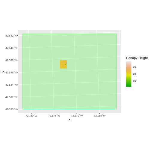
The plot above shows that the full CHM extent (plotted in green) is
much larger than the resulting cropped raster. Our new cropped CHM now
has the same extent as the aoi_boundary_HARV object that
was used as a crop extent (blue border below).
R
ggplot() +
  geom_raster(data = CHM_HARV_Cropped_df,
              aes(x = x, y = y, fill = HARV_chmCrop)) +
  geom_sf(data = aoi_boundary_HARV, color = "blue", fill = NA) +
  scale_fill_gradientn(name = "Canopy Height", colors = terrain.colors(10)) +
  coord_sf()
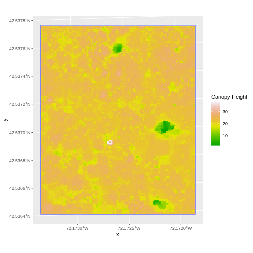
We can look at the extent of all of our other objects for this field site.
R
st_bbox(CHM_HARV)
OUTPUT
   xmin    ymin    xmax    ymax
 731453 4712471  733150 4713838
R
st_bbox(CHM_HARV_Cropped)
OUTPUT
   xmin    ymin    xmax    ymax
 732128 4713209  732251 4713359
R
st_bbox(aoi_boundary_HARV)
OUTPUT
     xmin      ymin      xmax      ymax
 732128.0 4713208.7  732251.1 4713359.2
R
st_bbox(plot_locations_sp_HARV)
OUTPUT
     xmin      ymin      xmax      ymax
 731405.3 4712845.0  732275.3 4713846.3
Our plot location extent is not the largest but is larger than the AOI Boundary. It would be nice to see our vegetation plot locations plotted on top of the Canopy Height Model information.
Challenge: Crop to Vector Points Extent
- Crop the Canopy Height Model to the extent of the study plot locations.
- Plot the vegetation plot location points on top of the Canopy Height Model.
R
CHM_plots_HARVcrop <- crop(x = CHM_HARV, y = plot_locations_sp_HARV)

CHM_plots_HARVcrop_df <- as.data.frame(CHM_plots_HARVcrop, xy = TRUE)

ggplot() +
  geom_raster(data = CHM_plots_HARVcrop_df,
              aes(x = x, y = y, fill = HARV_chmCrop)) +
  scale_fill_gradientn(name = "Canopy Height", colors = terrain.colors(10)) +
  geom_sf(data = plot_locations_sp_HARV) +
  coord_sf()
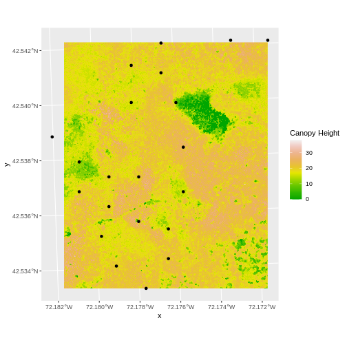
In the plot above, created in the challenge, all the vegetation plot locations (black dots) appear on the Canopy Height Model raster layer except for one. One is situated on the blank space to the left of the map. Why?
A modification of the first figure in this episode is below, showing
the relative extents of all the spatial objects. Notice that the extent
for our vegetation plot layer (black) extends further west than the
extent of our CHM raster (bright green). The crop()
function will make a raster extent smaller, it will not expand the
extent in areas where there are no data. Thus, the extent of our
vegetation plot layer will still extend further west than the extent of
our (cropped) raster data (dark green).
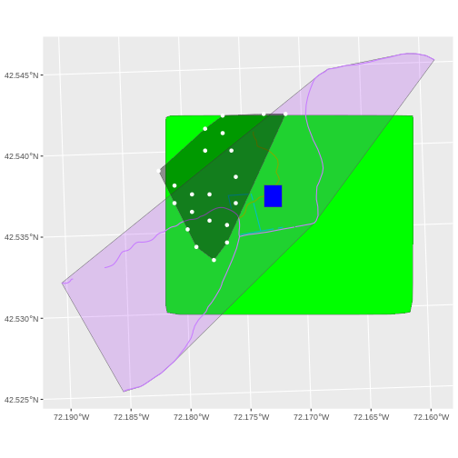
Define an Extent
So far, we have used a vector layer to crop the extent of a raster
dataset. Alternatively, we can also the ext() function to
define an extent to be used as a cropping boundary. This creates a new
object of class extent. Here we will provide the ext()
function our xmin, xmax, ymin, and ymax (in that order).
R
new_extent <- ext(732161.2, 732238.7, 4713249, 4713333)
class(new_extent)
OUTPUT
[1] "SpatExtent"
attr(,"package")
[1] "terra"
Data Tip
The extent can be created from a numeric vector (as shown above), a
matrix, or a list. For more details see the ext() function
help file (?terra::ext).
Once we have defined our new extent, we can use the
crop() function to crop our raster to this extent
object.
R
CHM_HARV_manual_cropped <- crop(x = CHM_HARV, y = new_extent)
To plot this data using ggplot() we need to convert it
to a dataframe.
R
CHM_HARV_manual_cropped_df <- as.data.frame(CHM_HARV_manual_cropped, xy = TRUE)
Now we can plot this cropped data. We will show the AOI boundary on the same plot for scale.
R
ggplot() +
  geom_sf(data = aoi_boundary_HARV, color = "blue", fill = NA) +
  geom_raster(data = CHM_HARV_manual_cropped_df,
              aes(x = x, y = y, fill = HARV_chmCrop)) +
  scale_fill_gradientn(name = "Canopy Height", colors = terrain.colors(10)) +
  coord_sf()
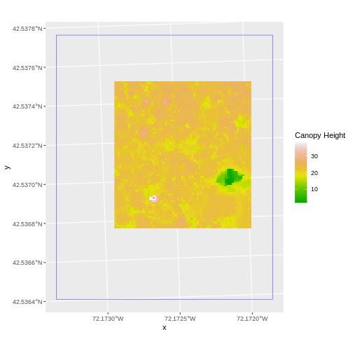
Extract Raster Pixels Values Using Vector Polygons
Often we want to extract values from a raster layer for particular locations - for example, plot locations that we are sampling on the ground. We can extract all pixel values within 20m of our x,y point of interest. These can then be summarized into some value of interest (e.g. mean, maximum, total).
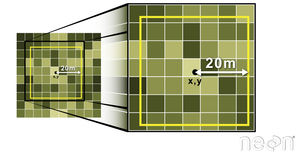 Image Source: National Ecological Observatory Network (NEON)
To do this in R, we use the extract() function. The
extract() function requires:
- The raster that we wish to extract values from,
- The vector layer containing the polygons that we wish to use as a boundary or boundaries,
- we can tell it to store the output values in a data frame using
raw = FALSE(this is optional).
We will begin by extracting all canopy height pixel values located
within our aoi_boundary_HARV polygon which surrounds the
tower located at the NEON Harvard Forest field site.
R
tree_height <- extract(x = CHM_HARV, y = aoi_boundary_HARV, raw = FALSE)

str(tree_height)
OUTPUT
'data.frame':	18450 obs. of  2 variables:
 $ ID          : num  1 1 1 1 1 1 1 1 1 1 ...
 $ HARV_chmCrop: num  21.2 23.9 23.8 22.4 23.9 ...
When we use the extract() function, R extracts the value
for each pixel located within the boundary of the polygon being used to
perform the extraction - in this case the aoi_boundary_HARV
object (a single polygon). Here, the function extracted values from
18,450 pixels.
We can create a histogram of tree height values within the boundary
to better understand the structure or height distribution of trees at
our site. We will use the column HARV_chmCrop from our data
frame as our x values, as this column represents the tree heights for
each pixel.
R
ggplot() +
  geom_histogram(data = tree_height, aes(x = HARV_chmCrop)) +
  ggtitle("Histogram of CHM Height Values (m)") +
  xlab("Tree Height") +
  ylab("Frequency of Pixels")
OUTPUT
`stat_bin()` using `bins = 30`. Pick better value with `binwidth`.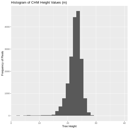
We can also use the summary() function to view
descriptive statistics including min, max, and mean height values. These
values help us better understand vegetation at our field site.
R
summary(tree_height$HARV_chmCrop)
OUTPUT
   Min. 1st Qu.  Median    Mean 3rd Qu.    Max.
   2.03   21.36   22.81   22.43   23.97   38.17
Summarize Extracted Raster Values
We often want to extract summary values from a raster. We can tell R
the type of summary statistic we are interested in using the
fun = argument. Let’s extract a mean height value for our
AOI.
R
mean_tree_height_AOI <- extract(x = CHM_HARV, y = aoi_boundary_HARV,
                                fun = mean)

mean_tree_height_AOI
OUTPUT
  ID HARV_chmCrop
1  1     22.43018
It appears that the mean height value, extracted from our LiDAR data derived canopy height model is 22.43 meters.
Extract Data using x,y Locations
We can also extract pixel values from a raster by defining a buffer
or area surrounding individual point locations using the
st_buffer() function. To do this we define the summary
argument (fun = mean) and the buffer distance
(dist = 20) which represents the radius of a circular
region around each point. By default, the units of the buffer are the
same units as the data’s CRS. All pixels that are touched by the buffer
region are included in the extract.
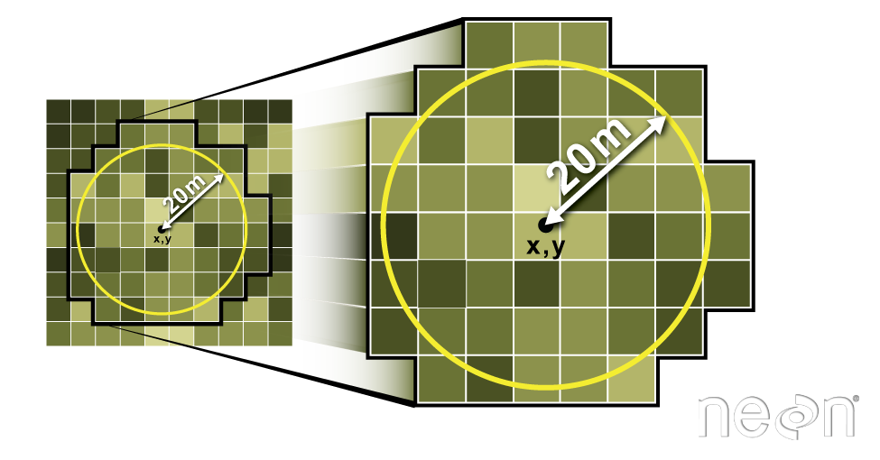 Image Source: National Ecological Observatory Network (NEON)
Let’s put this into practice by figuring out the mean tree height in
the 20m around the tower location (point_HARV).
R
mean_tree_height_tower <- extract(x = CHM_HARV,
                                  y = st_buffer(point_HARV, dist = 20),
                                  fun = mean)

mean_tree_height_tower
OUTPUT
  ID HARV_chmCrop
1  1     22.38806
Challenge: Extract Raster Height Values For Plot Locations
Use the plot locations object (
plot_locations_sp_HARV) to extract an average tree height for the area within 20m of each vegetation plot location in the study area. Because there are multiple plot locations, there will be multiple averages returned.Create a plot showing the mean tree height of each area.
R
# extract data at each plot location
mean_tree_height_plots_HARV <- extract(x = CHM_HARV,
                                       y = st_buffer(plot_locations_sp_HARV,
                                                     dist = 20),
                                       fun = mean)

# view data
mean_tree_height_plots_HARV
OUTPUT
   ID HARV_chmCrop
1   1          NaN
2   2     23.96756
3   3     22.34937
4   4     16.49739
5   5     21.54419
6   6     19.16772
7   7     20.61651
8   8     21.61439
9   9     12.23006
10 10     19.13398
11 11     21.36966
12 12     19.32084
13 13     17.25975
14 14     20.47120
15 15     12.68301
16 16     15.51888
17 17     18.90894
18 18     18.19369
19 19     19.67441
20 20     20.23245
21 21     20.44984
R
# plot data
ggplot(data = mean_tree_height_plots_HARV, aes(ID, HARV_chmCrop)) +
  geom_col() +
  ggtitle("Mean Tree Height at each Plot") +
  xlab("Plot ID") +
  ylab("Tree Height (m)")
WARNING
Warning: Removed 1 row containing missing values or values outside the scale range
(`geom_col()`).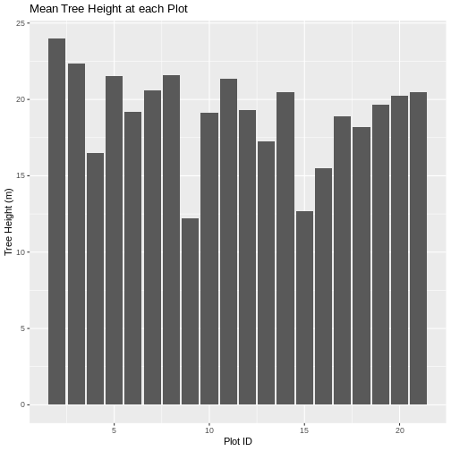
Key Points
- Use the
crop()function to crop a raster object. - Use the
extract()function to extract pixels from a raster object that fall within a particular extent boundary. - Use the
ext()function to define an extent.
Content from Raster Time Series Data
Last updated on 2024-10-15 | Edit this page
Overview
Questions
- How can I view and and plot data for different times of the year?
Objectives
- Understand the format of a time series raster dataset.
- Work with time series rasters.
- Import a set of rasters stored in a single directory.
- Create a multi-paneled plot.
- Convert character data to date format.
Things You’ll Need To Complete This Episode
See the lesson homepage for detailed information about the software, data, and other prerequisites you will need to work through the examples in this episode.
This episode covers how to work with and plot a raster time series, using an R raster object. It also covers practical assessment of data quality in remote sensing derived imagery.
About Raster Time Series Data
A raster data file can contain one single band or many bands. If the raster data contains imagery data, each band may represent reflectance for a different wavelength (color or type of light) or set of wavelengths - for example red, green and blue. A multi-band raster may two or more bands or layers of data collected at different times for the same extent (region) and of the same resolution. For this episode, we will work with a time series of normalized difference vegetation index (NDVI) and RGB data from the Harvard Forest site. We introduced the concepts of NDVI and RGB data in an earlier lesson and worked with an RGB RasterStack in the Work with Multi-band Rasters in R episode.
In this episode, we will:
- Import NDVI data in GeoTIFF format.
- Import, explore and plot NDVI data derived for several dates throughout the year.
- View the RGB imagery used to derived the NDVI time series to better understand unusual / outlier values.
RGB Data
While the NDVI data is a single band product, the RGB images that contain the red band used to derive NDVI, contain 3 (of the 7) 30m resolution bands available from Landsat data. The RGB directory contains RGB images for each time period that NDVI is available.
Getting Started
In this episode, we will use the terra,
scales, tidyr, and ggplot2
packages. Make sure you have them loaded.
R
library(terra)
library(scales)
library(tidyr)
library(ggplot2)
To begin, we will create a list of raster files using the
list.files() function. This list will be used to generate a
RasterStack. We will only add files that have a .tif
extension to our list. To do this, we will use the syntax
pattern=".tif$". If we specify
full.names = TRUE, the full path for each file will be
added to the list.
Data Tip
In the pattern above, the $ character represents the end
of a line. Using it ensures that our pattern will only match files that
end in .tif. This pattern matching uses a language called
“regular expressions”, which is beyond the scope of this workshop.
R
NDVI_HARV_path <- "data/NEON-DS-Landsat-NDVI/HARV/2011/NDVI"

all_NDVI_HARV <- list.files(NDVI_HARV_path,
                            full.names = TRUE,
                            pattern = ".tif$")
It’s a good idea to look at the file names that matched our search to make sure they meet our expectations.
R
all_NDVI_HARV
OUTPUT
 [1] "data/NEON-DS-Landsat-NDVI/HARV/2011/NDVI/005_HARV_ndvi_crop.tif"
 [2] "data/NEON-DS-Landsat-NDVI/HARV/2011/NDVI/037_HARV_ndvi_crop.tif"
 [3] "data/NEON-DS-Landsat-NDVI/HARV/2011/NDVI/085_HARV_ndvi_crop.tif"
 [4] "data/NEON-DS-Landsat-NDVI/HARV/2011/NDVI/133_HARV_ndvi_crop.tif"
 [5] "data/NEON-DS-Landsat-NDVI/HARV/2011/NDVI/181_HARV_ndvi_crop.tif"
 [6] "data/NEON-DS-Landsat-NDVI/HARV/2011/NDVI/197_HARV_ndvi_crop.tif"
 [7] "data/NEON-DS-Landsat-NDVI/HARV/2011/NDVI/213_HARV_ndvi_crop.tif"
 [8] "data/NEON-DS-Landsat-NDVI/HARV/2011/NDVI/229_HARV_ndvi_crop.tif"
 [9] "data/NEON-DS-Landsat-NDVI/HARV/2011/NDVI/245_HARV_ndvi_crop.tif"
[10] "data/NEON-DS-Landsat-NDVI/HARV/2011/NDVI/261_HARV_ndvi_crop.tif"
[11] "data/NEON-DS-Landsat-NDVI/HARV/2011/NDVI/277_HARV_ndvi_crop.tif"
[12] "data/NEON-DS-Landsat-NDVI/HARV/2011/NDVI/293_HARV_ndvi_crop.tif"
[13] "data/NEON-DS-Landsat-NDVI/HARV/2011/NDVI/309_HARV_ndvi_crop.tif"
Now we have a list of all GeoTIFF files in the NDVI directory for
Harvard Forest. The number at the start of the filenames represents the
julilan day. Next, we will create a stack of rasters from this list
using the rast() function. We worked with the
rast() function in an
earlier episode.
R
NDVI_HARV_stack <- rast(all_NDVI_HARV)
We can explore the GeoTIFF tags (the embedded metadata) in a stack
using the same syntax that we used on single-band raster objects in R
including: crs() (coordinate reference system),
ext() and res() (resolution; specifically
yres() and xres()).
R
crs(NDVI_HARV_stack, proj = TRUE)
OUTPUT
[1] "+proj=utm +zone=19 +ellps=WGS84 +units=m +no_defs"The CRS for our stack is
+proj=utm +zone=19 +ellps=WGS84 +units=m +no_defs. The CRS
is in UTM Zone 19. If you have completed the previous episodes in this
workshop, you may have noticed that the UTM zone for the NEON collected
remote sensing data was in Zone 18 rather than Zone 19. Why are the
Landsat data in Zone 19?
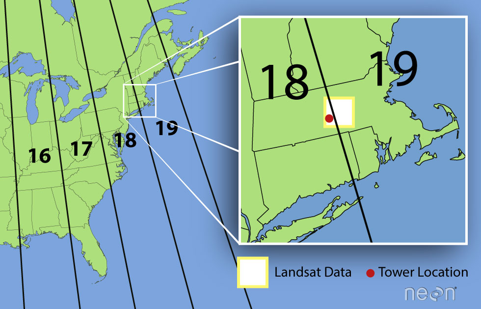
A Landsat scene is extremely wide - spanning over 170km north to south and 180km east to west. This means that Landsat data often cover multiple UTM zones. When the data are processed, the zone in which the majority of the data cover is the zone which is used for the final CRS. Thus, our field site at Harvard Forest is located in UTM Zone 18, but the Landsat data is in a CRS of UTM Zone 19.
Challenge: Raster Metadata
Investigate the metadata for our RasterStack and answer the following questions.
- What are the x and y resolution of the data?
- What units are the above resolution in?
R
ext(NDVI_HARV_stack)
OUTPUT
SpatExtent : 239415, 239535, 4714215, 4714365 (xmin, xmax, ymin, ymax)R
yres(NDVI_HARV_stack)
OUTPUT
[1] 30R
xres(NDVI_HARV_stack)
OUTPUT
[1] 30Plotting Time Series Data
Once we have created our RasterStack, we can visualize our data. We
can use the ggplot() command to create a multi-panelled
plot showing each band in our RasterStack. First we need to create a
data frame object. Because there are multiple columns in our data that
are not variables, we will tidy (or “pivot”) the data so that we have a
single column with the NDVI observations. We will use the function
pivot_longer() from the tidyr package to do
this:
R
NDVI_HARV_stack_df <- as.data.frame(NDVI_HARV_stack, xy = TRUE) %>%
    pivot_longer(-(x:y), names_to = "variable", values_to = "value")
Now we can plot our data using ggplot(). We want to
create a separate panel for each time point in our time series, so we
will use the facet_wrap() function to create a
multi-paneled plot:
R
ggplot() +
geom_raster(data = NDVI_HARV_stack_df , aes(x = x, y = y, fill = value)) +
facet_wrap(~ variable)

Look at the range of NDVI values observed in the plot above. We know that the accepted values for NDVI range from 0-1. Why does our data range from 0 - 10,000?
Scale Factors
The metadata for this NDVI data specifies a scale factor: 10,000. A scale factor is sometimes used to maintain smaller file sizes by removing decimal places. Storing data in integer format keeps files sizes smaller.
Let’s apply the scale factor before we go any further. Conveniently, we can quickly apply this factor using raster math on the entire stack as follows:
R
NDVI_HARV_stack <- NDVI_HARV_stack/10000
After applying our scale factor, we can recreate our plot using the same code we used above.
R
NDVI_HARV_stack_df <- as.data.frame(NDVI_HARV_stack, xy = TRUE) %>%
pivot_longer(-(x:y), names_to = "variable", values_to = "value")
ggplot() +
geom_raster(data = NDVI_HARV_stack_df , aes(x = x, y = y, fill = value)) +
facet_wrap(~variable)
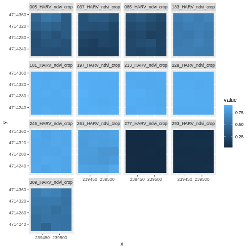
Take a Closer Look at Our Data
Let’s take a closer look at the plots of our data. Massachusetts, where the NEON Harvard Forest Field Site is located, has a fairly consistent fall, winter, spring, and summer season where vegetation turns green in the spring, continues to grow throughout the summer, and begins to change colors and senesce in the fall through winter. Do you notice anything that seems unusual about the patterns of greening and browning observed in the plots above?
Hint: the number after the “X” in each tile title is the Julian day which in this case represents the number of days into each year. If you are unfamiliar with Julian day, check out the NEON Data Skills Converting to Julian Day tutorial.
View Distribution of Raster Values
In the above exercise, we viewed plots of our NDVI time series and noticed a few images seem to be unusually light. However this was only a visual representation of potential issues in our data. What is another way we can look at these data that is quantitative?
Next we will use histograms to explore the distribution of NDVI values stored in each raster.
R
ggplot(NDVI_HARV_stack_df) +
geom_histogram(aes(value)) +
facet_wrap(~variable)
OUTPUT
`stat_bin()` using `bins = 30`. Pick better value with `binwidth`.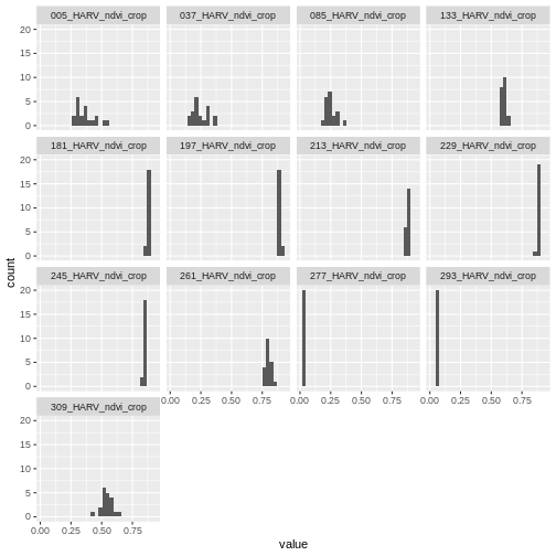
It seems like things get green in the spring and summer like we expect, but the data at Julian days 277 and 293 are unusual. It appears as if the vegetation got green in the spring, but then died back only to get green again towards the end of the year. Is this right?
Explore Unusual Data Patterns
The NDVI data that we are using comes from 2011, perhaps a strong freeze around Julian day 277 could cause a vegetation to senesce early, however in the eastern United States, it seems unusual that it would proceed to green up again shortly thereafter.
Let’s next view some temperature data for our field site to see whether there were some unusual fluctuations that may explain this pattern of greening and browning seen in the NDVI data. First we will read in the temperature data and preview the structure of that dataframe:
R
har_met_daily <-
read.csv("data/NEON-DS-Met-Time-Series/HARV/FisherTower-Met/hf001-06-daily-m.csv")
str(har_met_daily)
OUTPUT
'data.frame': 5345 obs. of 46 variables:
$ date : chr "2001-02-11" "2001-02-12" "2001-02-13" "2001-02-14" ...
$ jd : int 42 43 44 45 46 47 48 49 50 51 ...
$ airt : num -10.7 -9.8 -2 -0.5 -0.4 -3 -4.5 -9.9 -4.5 3.2 ...
$ f.airt : chr "" "" "" "" ...
$ airtmax : num -6.9 -2.4 5.7 1.9 2.4 1.3 -0.7 -3.3 0.7 8.9 ...
$ f.airtmax: chr "" "" "" "" ...
$ airtmin : num -15.1 -17.4 -7.3 -5.7 -5.7 -9 -12.7 -17.1 -11.7 -1.3 ...
$ f.airtmin: chr "" "" "" "" ...
$ rh : int 40 45 70 78 69 82 66 51 57 62 ...
$ f.rh : chr "" "" "" "" ...
$ rhmax : int 58 85 100 100 100 100 100 71 81 78 ...
$ f.rhmax : chr "" "" "" "" ...
$ rhmin : int 22 14 34 59 37 46 30 34 37 42 ...
$ f.rhmin : chr "" "" "" "" ...
$ dewp : num -22.2 -20.7 -7.6 -4.1 -6 -5.9 -10.8 -18.5 -12 -3.5 ...
$ f.dewp : chr "" "" "" "" ...
$ dewpmax : num -16.8 -9.2 -4.6 1.9 2 -0.4 -0.7 -14.4 -4 0.6 ...
$ f.dewpmax: chr "" "" "" "" ...
$ dewpmin : num -25.7 -27.9 -10.2 -10.2 -12.1 -10.6 -25.4 -25 -16.5 -5.7 ...
$ f.dewpmin: chr "" "" "" "" ...
$ prec : num 0 0 0 6.9 0 2.3 0 0 0 0 ...
$ f.prec : chr "" "" "" "" ...
$ slrt : num 14.9 14.8 14.8 2.6 10.5 6.4 10.3 15.5 15 7.7 ...
$ f.slrt : chr "" "" "" "" ...
$ part : num NA NA NA NA NA NA NA NA NA NA ...
$ f.part : chr "M" "M" "M" "M" ...
$ netr : num NA NA NA NA NA NA NA NA NA NA ...
$ f.netr : chr "M" "M" "M" "M" ...
$ bar : int 1025 1033 1024 1016 1010 1016 1008 1022 1022 1017 ...
$ f.bar : chr "" "" "" "" ...
$ wspd : num 3.3 1.7 1.7 2.5 1.6 1.1 3.3 2 2.5 2 ...
$ f.wspd : chr "" "" "" "" ...
$ wres : num 2.9 0.9 0.9 1.9 1.2 0.5 3 1.9 2.1 1.8 ...
$ f.wres : chr "" "" "" "" ...
$ wdir : int 287 245 278 197 300 182 281 272 217 218 ...
$ f.wdir : chr "" "" "" "" ...
$ wdev : int 27 55 53 38 40 56 24 24 31 27 ...
$ f.wdev : chr "" "" "" "" ...
$ gspd : num 15.4 7.2 9.6 11.2 12.7 5.8 16.9 10.3 11.1 10.9 ...
$ f.gspd : chr "" "" "" "" ...
$ s10t : num NA NA NA NA NA NA NA NA NA NA ...
$ f.s10t : chr "M" "M" "M" "M" ...
$ s10tmax : num NA NA NA NA NA NA NA NA NA NA ...
$ f.s10tmax: chr "M" "M" "M" "M" ...
$ s10tmin : num NA NA NA NA NA NA NA NA NA NA ...
$ f.s10tmin: chr "M" "M" "M" "M" ...The date column is currently coded as a character. We
want to be able to treat it as a date, so we will use the
as.Date() function to convert it. We need to tell R what
format the data is in. Our dates are YYY-MM-DD, which is represented by
R as %Y-%m-%d.
R
har_met_daily$date <- as.Date(har_met_daily$date, format = "%Y-%m-%d")
We only want to look at the data from 2011:
R
yr_11_daily_avg <- har_met_daily %>%
filter(between(date, as.Date('2011-01-01'), as.Date('2011-12-31')))
Now we can plot the air temperature (the airt column) by
Julian day (the jd column):
R
ggplot() +
geom_point(data = yr_11_daily_avg, aes(jd, airt)) +
ggtitle("Daily Mean Air Temperature",
subtitle = "NEON Harvard Forest Field Site") +
xlab("Julian Day 2011") +
ylab("Mean Air Temperature (C)")
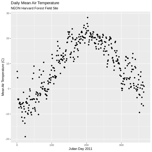
There are no significant peaks or dips in the temperature during the late summer or early fall time period that might account for patterns seen in the NDVI data. Let’s have a look at the source Landsat imagery that was partially used used to derive our NDVI rasters to try to understand what appear to be outlier NDVI values.
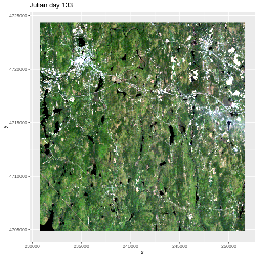
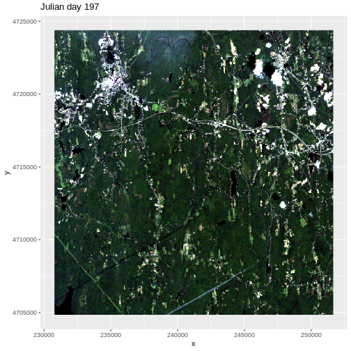
Challenge: Examine RGB Raster Files
Plot the RGB images for the Julian days 277 and 293. Compare those with the RGB plots for Julian days 133 and 197 (shown above). Does the RGB imagery from these two days explain the low NDVI values observed on these days?
First we need to load in the RGB data for Julian day 277 and look at its metadata.
R
RGB_277 <- rast("data/NEON-DS-Landsat-NDVI/HARV/2011/RGB/277_HARV_landRGB.tif")
# NOTE: Fix the bands' names so they don't start with a number!
names(RGB_277) <- paste0("X", names(RGB_277))
RGB_277
OUTPUT
class : SpatRaster
dimensions : 652, 696, 3 (nrow, ncol, nlyr)
resolution : 30, 30 (x, y)
extent : 230775, 251655, 4704825, 4724385 (xmin, xmax, ymin, ymax)
coord. ref. : WGS 84 / UTM zone 19N (EPSG:32619)
source : 277_HARV_landRGB.tif
names : X277_HARV_landRGB_1, X277_HARV_landRGB_2, X277_HARV_landRGB_3
min values : 26, 29, 79
max values : 255, 255, 255 The RGB data has a max value of 255, but we need our color intensity to be between 0 and 1, so we will divide our RasterStack object by 255.
R
RGB_277 <- RGB_277/255
Next we convert it to a dataframe.
R
RGB_277_df <- as.data.frame(RGB_277, xy = TRUE)
We create RGB colors from the three channels:
R
RGB_277_df$rgb <-
with(RGB_277_df, rgb(X277_HARV_landRGB_1, X277_HARV_landRGB_2,
X277_HARV_landRGB_3, 1))
Finally, we can plot the RGB data for Julian day 277.
R
ggplot() +
geom_raster(data=RGB_277_df, aes(x, y), fill=RGB_277_df$rgb) +
ggtitle("Julian day 277")
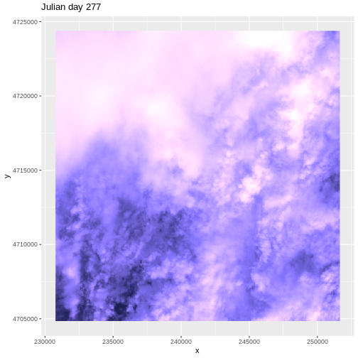
We then do the same steps for Julian day 293
R
# Julian day 293
RGB_293 <- rast("data/NEON-DS-Landsat-NDVI/HARV/2011/RGB/293_HARV_landRGB.tif")
names(RGB_293) <- paste0("X", names(RGB_293))
RGB_293 <- RGB_293/255
RGB_293_df <- as.data.frame(RGB_293, xy = TRUE)
RGB_293_df$rgb <-
with(RGB_293_df, rgb(X293_HARV_landRGB_1, X293_HARV_landRGB_2,
X293_HARV_landRGB_3,1))
ggplot() +
geom_raster(data = RGB_293_df, aes(x, y), fill = RGB_293_df$rgb) +
ggtitle("Julian day 293")
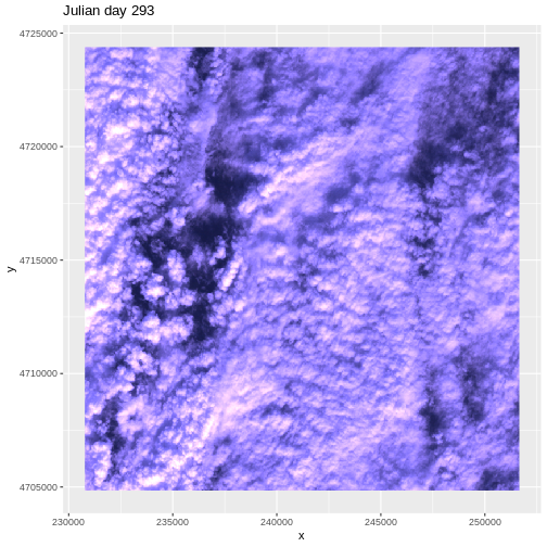
This example highlights the importance of exploring the source of a derived data product. In this case, the NDVI data product was created using Landsat imagery - specifically the red and near-infrared bands. When we look at the RGB collected at Julian days 277 and 293 we see that most of the image is filled with clouds. The very low NDVI values resulted from cloud cover — a common challenge that we encounter when working with satellite remote sensing imagery.
Key Points
- Use the
list.files()function to get a list of filenames matching a specific pattern. - Use the
facet_wrap()function to create multi-paneled plots withggplot2. - Use the
as.Date()function to convert data to date format.
Content from Create Publication-quality Graphics
Last updated on 2024-10-15 | Edit this page
Overview
Questions
- How can I create a publication-quality graphic and customize plot parameters?
Objectives
- Assign custom names to bands in a RasterStack.
- Customize raster plots using the
ggplot2package.
Things You’ll Need To Complete This Episode
See the lesson homepage for detailed information about the software, data, and other prerequisites you will need to work through the examples in this episode.
This episode covers how to customize your raster plots using the
ggplot2 package in R to create publication-quality
plots.
Before and After
In the previous episode, we
learned how to plot multi-band raster data in R using the
facet_wrap() function. This created a separate panel in our
plot for each raster band. The plot we created together is shown
below:
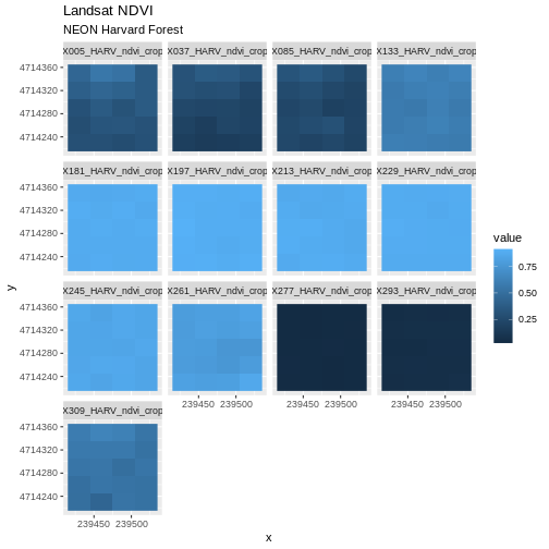
Although this plot is informative, it isn’t something we would expect to see in a journal publication. The x and y-axis labels aren’t informative. There is a lot of unnecessary gray background and the titles of each panel don’t clearly state that the number refers to the Julian day the data was collected. In this episode, we will customize this plot above to produce a publication quality graphic. We will go through these steps iteratively. When we’re done, we will have created the plot shown below.
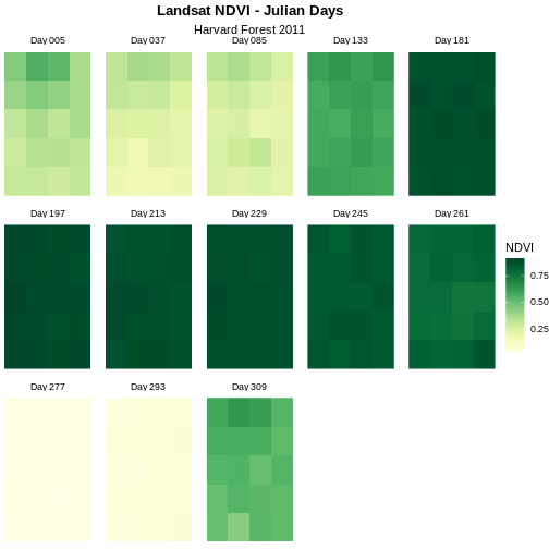
Adjust the Plot Theme
The first thing we will do to our plot remove the x and y-axis labels
and axis ticks, as these are unnecessary and make our plot look messy.
We can do this by setting the plot theme to void.
R
ggplot() +
geom_raster(data = NDVI_HARV_stack_df , aes(x = x, y = y, fill = value)) +
facet_wrap(~variable) +
ggtitle("Landsat NDVI", subtitle = "NEON Harvard Forest") +
theme_void()
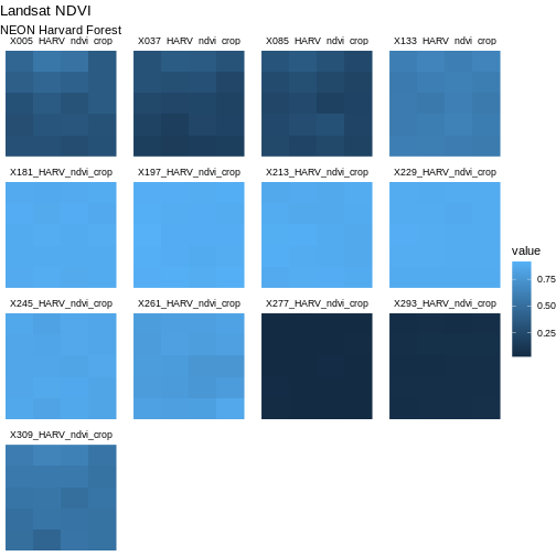
Next we will center our plot title and subtitle. We need to do this
after the theme_void() layer, because R
interprets the ggplot layers in order. If we first tell R
to center our plot title, and then set the theme to void,
any adjustments we’ve made to the plot theme will be over-written by the
theme_void() function. So first we make the theme
void and then we center the title. We center both the title
and subtitle by using the theme() function and setting the
hjust parameter to 0.5. The hjust parameter
stands for “horizontal justification” and takes any value between 0 and
1. A setting of 0 indicates left justification and a setting of 1
indicates right justification.
R
ggplot() +
geom_raster(data = NDVI_HARV_stack_df , aes(x = x, y = y, fill = value)) +
facet_wrap(~variable) +
ggtitle("Landsat NDVI", subtitle = "NEON Harvard Forest") +
theme_void() +
theme(plot.title = element_text(hjust = 0.5),
plot.subtitle = element_text(hjust = 0.5))

Challenge
Change the plot title (but not the subtitle) to bold font. You can (and should!) use the help menu in RStudio or any internet resources to figure out how to change this setting.
Learners can find this information in the help files for the
theme() function. The parameter to set is called
face.
R
ggplot() +
geom_raster(data = NDVI_HARV_stack_df,
aes(x = x, y = y, fill = value)) +
facet_wrap(~ variable) +
ggtitle("Landsat NDVI", subtitle = "NEON Harvard Forest") +
theme_void() +
theme(plot.title = element_text(hjust = 0.5, face = "bold"),
plot.subtitle = element_text(hjust = 0.5))

Adjust the Color Ramp
Next, let’s adjust the color ramp used to render the rasters. First,
we can change the blue color ramp to a green one that is more visually
suited to our NDVI (greenness) data using the
colorRampPalette() function in combination with
colorBrewer which requires loading the
RColorBrewer library. Then we use
scale_fill_gradientn to pass the list of colours (here 20
different colours) to ggplot.
First we need to create a set of colors to use. We will select a set of nine colors from the “YlGn” (yellow-green) color palette. This returns a set of hex color codes:
R
library(RColorBrewer)
brewer.pal(9, "YlGn")
OUTPUT
[1] "#FFFFE5" "#F7FCB9" "#D9F0A3" "#ADDD8E" "#78C679" "#41AB5D" "#238443"
[8] "#006837" "#004529"Then we will pass those color codes to the
colorRampPalette function, which will interpolate from
those colors a more nuanced color range.
R
green_colors <- brewer.pal(9, "YlGn") %>%
colorRampPalette()
We can tell the colorRampPalette() function how many
discrete colors within this color range to create. In our case, we will
use 20 colors when we plot our graphic.
R
ggplot() +
geom_raster(data = NDVI_HARV_stack_df , aes(x = x, y = y, fill = value)) +
facet_wrap(~variable) +
ggtitle("Landsat NDVI", subtitle = "NEON Harvard Forest") +
theme_void() +
theme(plot.title = element_text(hjust = 0.5, face = "bold"),
plot.subtitle = element_text(hjust = 0.5)) +
scale_fill_gradientn(name = "NDVI", colours = green_colors(20))
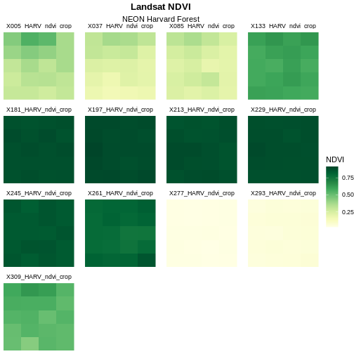
The yellow to green color ramp visually represents NDVI well given it’s a measure of greenness. Someone looking at the plot can quickly understand that pixels that are more green have a higher NDVI value.
Data Tip
For all of the brewer.pal ramp names see the brewerpal
page.
Data Tip
Cynthia Brewer, the creator of ColorBrewer, offers an online tool to help choose suitable color ramps, or to create your own. ColorBrewer 2.0; Color Advise for Cartography
Refine Plot & Tile Labels
Next, let’s label each panel in our plot with the Julian day that the
raster data for that panel was collected. The current names come from
the band “layer names”” stored in the RasterStack and the
first part of each name is the Julian day.
To create a more meaningful label we can remove the “x” and replace
it with “day” using the gsub() function in R. The syntax is
as follows:
gsub("StringToReplace", "TextToReplaceIt", object).
First let’s remove “_HARV_NDVI_crop” from each label to make the
labels shorter and remove repetition. To illustrate how this works, we
will first look at the names for our NDVI_HARV_stack
object:
R
names(NDVI_HARV_stack)
OUTPUT
[1] "X005_HARV_ndvi_crop" "X037_HARV_ndvi_crop" "X085_HARV_ndvi_crop"
[4] "X133_HARV_ndvi_crop" "X181_HARV_ndvi_crop" "X197_HARV_ndvi_crop"
[7] "X213_HARV_ndvi_crop" "X229_HARV_ndvi_crop" "X245_HARV_ndvi_crop"
[10] "X261_HARV_ndvi_crop" "X277_HARV_ndvi_crop" "X293_HARV_ndvi_crop"
[13] "X309_HARV_ndvi_crop"Now we will use the gsub() function to find the
character string “_HARV_ndvi_crop” and replace it with a blank string
(““). We will assign this output to a new object
(raster_names) and look at that object to make sure our
code is doing what we want it to.
R
raster_names <- names(NDVI_HARV_stack)
raster_names <- gsub("_HARV_ndvi_crop", "", raster_names)
raster_names
OUTPUT
[1] "X005" "X037" "X085" "X133" "X181" "X197" "X213" "X229" "X245" "X261"
[11] "X277" "X293" "X309"So far so good. Now we will use gsub() again to replace
the “X” with the word “Day” followed by a space.
R
raster_names <- gsub("X", "Day ", raster_names)
raster_names
OUTPUT
[1] "Day 005" "Day 037" "Day 085" "Day 133" "Day 181" "Day 197" "Day 213"
[8] "Day 229" "Day 245" "Day 261" "Day 277" "Day 293" "Day 309"Our labels look good now. Let’s reassign them to our
all_NDVI_HARV object:
R
labels_names <- setNames(raster_names, unique(NDVI_HARV_stack_df$variable))
Once the names for each band have been reassigned, we can render our
plot with the new labels using alabeller.
R
ggplot() +
geom_raster(data = NDVI_HARV_stack_df , aes(x = x, y = y, fill = value)) +
facet_wrap(~variable, labeller = labeller(variable = labels_names)) +
ggtitle("Landsat NDVI", subtitle = "NEON Harvard Forest") +
theme_void() +
theme(plot.title = element_text(hjust = 0.5, face = "bold"),
plot.subtitle = element_text(hjust = 0.5)) +
scale_fill_gradientn(name = "NDVI", colours = green_colors(20))

Change Layout of Panels
We can adjust the columns of our plot by setting the number of
columns ncol and the number of rows nrow in
facet_wrap. Let’s make our plot so that it has a width of
five panels.
R
ggplot() +
geom_raster(data = NDVI_HARV_stack_df , aes(x = x, y = y, fill = value)) +
facet_wrap(~variable, ncol = 5,
labeller = labeller(variable = labels_names)) +
ggtitle("Landsat NDVI", subtitle = "NEON Harvard Forest") +
theme_void() +
theme(plot.title = element_text(hjust = 0.5, face = "bold"),
plot.subtitle = element_text(hjust = 0.5)) +
scale_fill_gradientn(name = "NDVI", colours = green_colors(20))
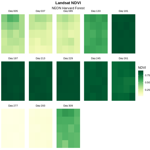
Now we have a beautiful, publication quality plot!
Challenge: Divergent Color Ramps
When we used the gsub() function to modify the tile
labels we replaced the beginning of each tile title with “Day”. A more
descriptive name could be “Julian Day”. Update the plot above with the
following changes:
- Label each tile “Julian Day” with the julian day value following.
- Change the color ramp to a divergent brown to green color ramp.
Questions: Does having a divergent color ramp represent the data better than a sequential color ramp (like “YlGn”)? Can you think of other data sets where a divergent color ramp may be best?
R
raster_names <- gsub("Day","Julian Day ", raster_names)
labels_names <- setNames(raster_names, unique(NDVI_HARV_stack_df$variable))
brown_green_colors <- colorRampPalette(brewer.pal(9, "BrBG"))
ggplot() +
geom_raster(data = NDVI_HARV_stack_df , aes(x = x, y = y, fill = value)) +
facet_wrap(~variable, ncol = 5, labeller = labeller(variable = labels_names)) +
ggtitle("Landsat NDVI - Julian Days", subtitle = "Harvard Forest 2011") +
theme_void() +
theme(plot.title = element_text(hjust = 0.5, face = "bold"),
plot.subtitle = element_text(hjust = 0.5)) +
scale_fill_gradientn(name = "NDVI", colours = brown_green_colors(20))
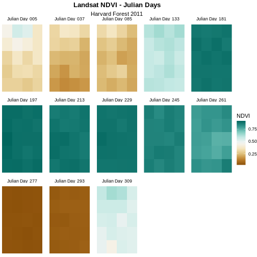
For NDVI data, the sequential color ramp is better than the divergent as it is more akin to the process of greening up, which starts off at one end and just keeps increasing.
Key Points
- Use the
theme_void()function for a clean background to your plot. - Use the
element_text()function to adjust text size, font, and position. - Use the
brewer.pal()function to create a custom color palette. - Use the
gsub()function to do pattern matching and replacement in text.
Content from Derive Values from Raster Time Series
Last updated on 2024-10-15 | Edit this page
Overview
Questions
- How can I calculate, extract, and export summarized raster pixel data?
Objectives
- Extract summary pixel values from a raster.
- Save summary values to a .csv file.
- Plot summary pixel values using
ggplot(). - Compare NDVI values between two different sites.
Things You’ll Need To Complete This Episode
See the lesson homepage for detailed information about the software, data, and other prerequisites you will need to work through the examples in this episode.
In this episode, we will extract NDVI values from a raster time
series dataset and plot them using the ggplot2 package.
Extract Summary Statistics From Raster Data
We often want to extract summary values from raster data. For example, we might want to understand overall greeness across a field site or at each plot within a field site. These values can then be compared between different field sites and combined with other related metrics to support modeling and further analysis.
Calculate Average NDVI
Our goal in this episode is to create a dataframe that contains a single, mean NDVI value for each raster in our time series. This value represents the mean NDVI value for this area on a given day.
We can calculate the mean for each raster using the
global() function. The global() function
produces a named numeric vector, where each value is associated with the
name of raster stack it was derived from.
R
avg_NDVI_HARV <- global(NDVI_HARV_stack, mean)
avg_NDVI_HARV
OUTPUT
mean
X005_HARV_ndvi_crop 0.365150
X037_HARV_ndvi_crop 0.242645
X085_HARV_ndvi_crop 0.251390
X133_HARV_ndvi_crop 0.599300
X181_HARV_ndvi_crop 0.878725
X197_HARV_ndvi_crop 0.893250
X213_HARV_ndvi_crop 0.878395
X229_HARV_ndvi_crop 0.881505
X245_HARV_ndvi_crop 0.850120
X261_HARV_ndvi_crop 0.796360
X277_HARV_ndvi_crop 0.033050
X293_HARV_ndvi_crop 0.056895
X309_HARV_ndvi_crop 0.541130The output is a data frame (othewise, we could use
as.data.frame()). It’s a good idea to view the first few
rows of our data frame with head() to make sure the
structure is what we expect.
R
head(avg_NDVI_HARV)
OUTPUT
mean
X005_HARV_ndvi_crop 0.365150
X037_HARV_ndvi_crop 0.242645
X085_HARV_ndvi_crop 0.251390
X133_HARV_ndvi_crop 0.599300
X181_HARV_ndvi_crop 0.878725
X197_HARV_ndvi_crop 0.893250We now have a data frame with row names that are based on the original file name and a mean NDVI value for each file. Next, let’s clean up the column names in our data frame to make it easier for colleagues to work with our code.
Let’s change the NDVI column name to meanNDVI.
R
names(avg_NDVI_HARV) <- "meanNDVI"
head(avg_NDVI_HARV)
OUTPUT
meanNDVI
X005_HARV_ndvi_crop 0.365150
X037_HARV_ndvi_crop 0.242645
X085_HARV_ndvi_crop 0.251390
X133_HARV_ndvi_crop 0.599300
X181_HARV_ndvi_crop 0.878725
X197_HARV_ndvi_crop 0.893250The new column name doesn’t reminds us what site our data are from. While we are only working with one site now, we might want to compare several sites worth of data in the future. Let’s add a column to our dataframe called “site”.
R
avg_NDVI_HARV$site <- "HARV"
We can populate this column with the site name - HARV. Let’s also create a year column and populate it with 2011 - the year our data were collected.
R
avg_NDVI_HARV$year <- "2011"
head(avg_NDVI_HARV)
OUTPUT
meanNDVI site year
X005_HARV_ndvi_crop 0.365150 HARV 2011
X037_HARV_ndvi_crop 0.242645 HARV 2011
X085_HARV_ndvi_crop 0.251390 HARV 2011
X133_HARV_ndvi_crop 0.599300 HARV 2011
X181_HARV_ndvi_crop 0.878725 HARV 2011
X197_HARV_ndvi_crop 0.893250 HARV 2011We now have a dataframe that contains a row for each raster file
processed, and columns for meanNDVI, site, and
year.
Extract Julian Day from row names
We’d like to produce a plot where Julian days (the numeric day of the year, 0 - 365/366) are on the x-axis and NDVI is on the y-axis. To create this plot, we’ll need a column that contains the Julian day value.
One way to create a Julian day column is to use gsub()
on the file name in each row. We can replace both the X and
the _HARV_NDVI_crop to extract the Julian Day value, just
like we did in the previous
episode.
This time we will use one additional trick to do both of these steps
at the same time. The vertical bar character ( | ) is
equivalent to the word “or”. Using this character in our search pattern
allows us to search for more than one pattern in our text strings.
R
julianDays <- gsub("X|_HARV_ndvi_crop", "", row.names(avg_NDVI_HARV))
julianDays
OUTPUT
[1] "005" "037" "085" "133" "181" "197" "213" "229" "245" "261" "277" "293"
[13] "309"Now that we’ve extracted the Julian days from our row names, we can add that data to the data frame as a column called “julianDay”.
R
avg_NDVI_HARV$julianDay <- julianDays
Let’s check the class of this new column:
R
class(avg_NDVI_HARV$julianDay)
OUTPUT
[1] "character"Convert Julian Day to Date Class
Currently, the values in the Julian day column are stored as class
character. Storing this data as a date object is better -
for plotting, data subsetting and working with our data. Let’s convert.
We worked with data conversions in an
earlier episode. For an introduction to date-time classes, see the
NEON Data Skills tutorial Convert
Date & Time Data from Character Class to Date-Time Class (POSIX) in
R.
To convert a Julian day number to a date class, we need to set the origin, which is the day that our Julian days start counting from. Our data is from 2011 and we know that the USGS Landsat Team created Julian day values for this year. Therefore, the first day or “origin” for our Julian day count is 01 January 2011.
R
origin <- as.Date("2011-01-01")
Next we convert the julianDay column from character to
integer.
R
avg_NDVI_HARV$julianDay <- as.integer(avg_NDVI_HARV$julianDay)
Once we set the Julian day origin, we can add the Julian day value (as an integer) to the origin date.
Note that when we convert our integer class julianDay
values to dates, we subtracted 1. This is because the origin day is 01
January 2011, so the extracted day is 01. The Julian Day (or year day)
for this is also 01. When we convert from the integer 05
julianDay value (indicating 5th of January), we cannot
simply add origin + julianDay because
01 + 05 = 06 or 06 January 2011. To correct, this error we
then subtract 1 to get the correct day, January 05 2011.
R
avg_NDVI_HARV$Date<- origin + (avg_NDVI_HARV$julianDay - 1)
head(avg_NDVI_HARV$Date)
OUTPUT
[1] "2011-01-05" "2011-02-06" "2011-03-26" "2011-05-13" "2011-06-30"
[6] "2011-07-16"Since the origin date was originally set as a Date class object, the
new Date column is also stored as class
Date.
R
class(avg_NDVI_HARV$Date)
OUTPUT
[1] "Date"Challenge: NDVI for the San Joaquin Experimental Range
We often want to compare two different sites. The National Ecological Observatory Network (NEON) also has a field site in Southern California at the San Joaquin Experimental Range (SJER).
For this challenge, create a dataframe containing the mean NDVI
values and the Julian days the data was collected (in date format) for
the NEON San Joaquin Experimental Range field site. NDVI data for SJER
are located in the NEON-DS-Landsat-NDVI/SJER/2011/NDVI
directory.
First we will read in the NDVI data for the SJER field site.
R
NDVI_path_SJER <- "data/NEON-DS-Landsat-NDVI/SJER/2011/NDVI"
all_NDVI_SJER <- list.files(NDVI_path_SJER,
full.names = TRUE,
pattern = ".tif$")
NDVI_stack_SJER <- rast(all_NDVI_SJER)
names(NDVI_stack_SJER) <- paste0("X", names(NDVI_stack_SJER))
NDVI_stack_SJER <- NDVI_stack_SJER/10000
Then we can calculate the mean values for each day and put that in a dataframe.
R
avg_NDVI_SJER <- as.data.frame(global(NDVI_stack_SJER, mean))
Next we rename the NDVI column, and add site and year columns to our data.
R
names(avg_NDVI_SJER) <- "meanNDVI"
avg_NDVI_SJER$site <- "SJER"
avg_NDVI_SJER$year <- "2011"
Now we will create our Julian day column
R
julianDays_SJER <- gsub("X|_SJER_ndvi_crop", "", row.names(avg_NDVI_SJER))
origin <- as.Date("2011-01-01")
avg_NDVI_SJER$julianDay <- as.integer(julianDays_SJER)
avg_NDVI_SJER$Date <- origin + (avg_NDVI_SJER$julianDay - 1)
head(avg_NDVI_SJER)
OUTPUT
meanNDVI site year julianDay Date
X014_SJER_ndvi_crop 0.048216 SJER 2011 14 2011-01-14
X046_SJER_ndvi_crop 0.529780 SJER 2011 46 2011-02-15
X062_SJER_ndvi_crop 0.554368 SJER 2011 62 2011-03-03
X094_SJER_ndvi_crop 0.601096 SJER 2011 94 2011-04-04
X110_SJER_ndvi_crop 0.555836 SJER 2011 110 2011-04-20
X126_SJER_ndvi_crop 0.538336 SJER 2011 126 2011-05-06Plot NDVI Using ggplot
We now have a clean dataframe with properly scaled NDVI and Julian days. Let’s plot our data.
R
ggplot(avg_NDVI_HARV, aes(julianDay, meanNDVI)) +
geom_point() +
ggtitle("Landsat Derived NDVI - 2011",
subtitle = "NEON Harvard Forest Field Site") +
xlab("Julian Days") + ylab("Mean NDVI")
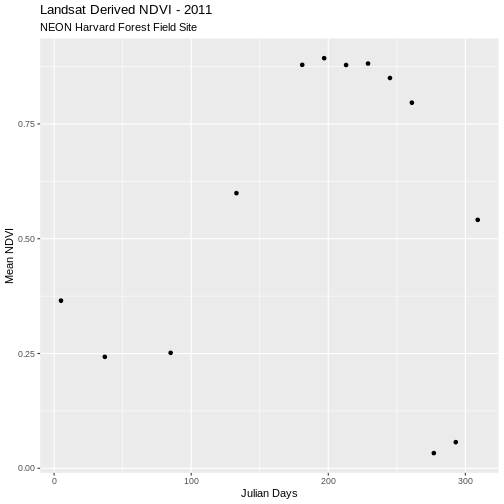
Challenge: Plot San Joaquin Experimental Range Data
Create a complementary plot for the SJER data. Plot the data points in a different color.
R
ggplot(avg_NDVI_SJER, aes(julianDay, meanNDVI)) +
geom_point(colour = "SpringGreen4") +
ggtitle("Landsat Derived NDVI - 2011", subtitle = "NEON SJER Field Site") +
xlab("Julian Day") + ylab("Mean NDVI")
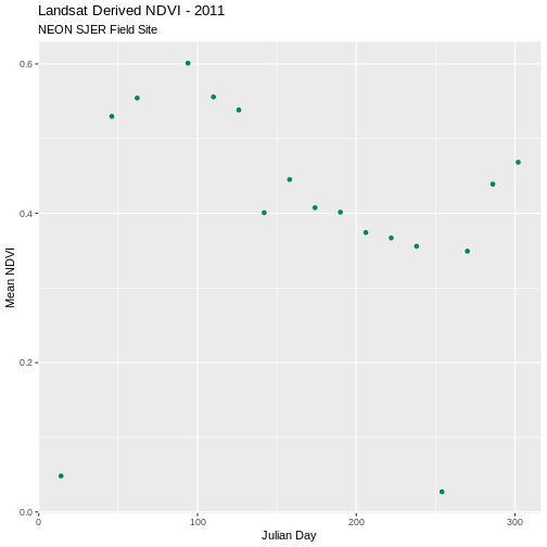
Compare NDVI from Two Different Sites in One Plot
Comparison of plots is often easiest when both plots are side by side. Or, even better, if both sets of data are plotted in the same plot. We can do this by merging the two data sets together. The date frames must have the same number of columns and exact same column names to be merged.
R
NDVI_HARV_SJER <- rbind(avg_NDVI_HARV, avg_NDVI_SJER)
Now we can plot both datasets on the same plot.
R
ggplot(NDVI_HARV_SJER, aes(x = julianDay, y = meanNDVI, colour = site)) +
geom_point(aes(group = site)) +
geom_line(aes(group = site)) +
ggtitle("Landsat Derived NDVI - 2011",
subtitle = "Harvard Forest vs San Joaquin") +
xlab("Julian Day") + ylab("Mean NDVI")
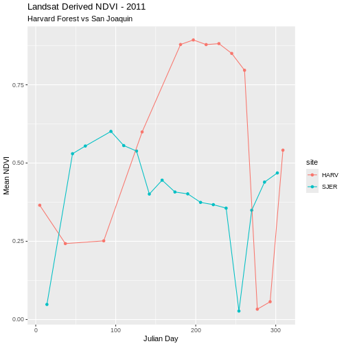
Challenge: Plot NDVI with date
Plot the SJER and HARV data in one plot but use date, rather than Julian day, on the x-axis.
R
ggplot(NDVI_HARV_SJER, aes(x = Date, y = meanNDVI, colour = site)) +
geom_point(aes(group = site)) +
geom_line(aes(group = site)) +
ggtitle("Landsat Derived NDVI - 2011",
subtitle = "Harvard Forest vs San Joaquin") +
xlab("Date") + ylab("Mean NDVI")
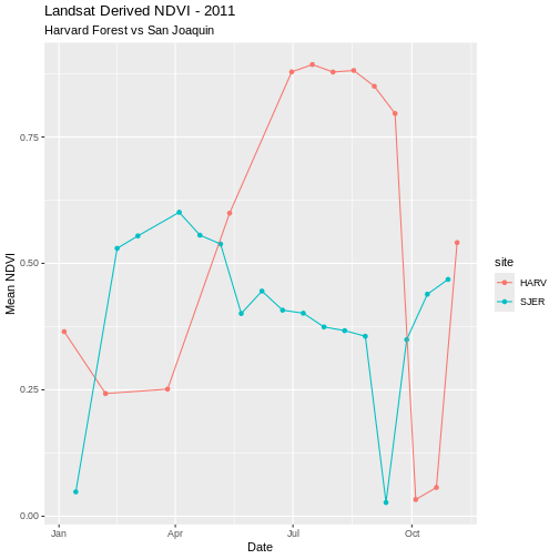
Remove Outlier Data
As we look at these plots we see variation in greenness across the year. However, the pattern is interrupted by a few points where NDVI quickly drops towards 0 during a time period when we might expect the vegetation to have a higher greenness value. Is the vegetation truly senescent or gone or are these outlier values that should be removed from the data?
We’ve seen in an earlier episode that data points with very low NDVI values can be associated with images that are filled with clouds. Thus, we can attribute the low NDVI values to high levels of cloud cover. Is the same thing happening at SJER?
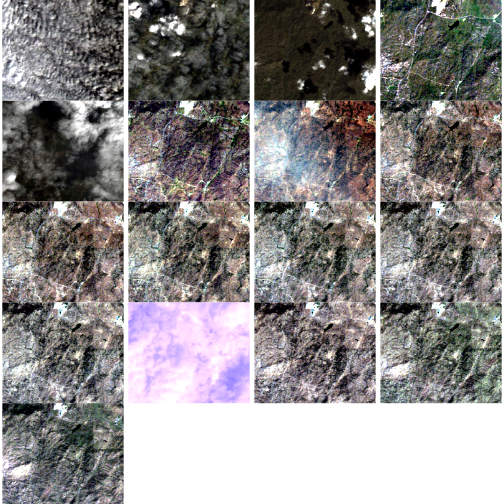
Without significant additional processing, we will not be able to retrieve a strong reflection from vegetation, from a remotely sensed image that is predominantly cloud covered. Thus, these points are likely bad data points. Let’s remove them.
First, we will identify the good data points that should be retained. One way to do this is by identifying a threshold value. All values below that threshold will be removed from our analysis. We will use 0.1 as an example for this episode. We can then use the subset function to remove outlier datapoints (below our identified threshold).
Data Tip
Thresholding, or removing outlier data, can be tricky business. In this case, we can be confident that some of our NDVI values are not valid due to cloud cover. However, a threshold value may not always be sufficient given that 0.1 could be a valid NDVI value in some areas. This is where decision-making should be fueled by practical scientific knowledge of the data and the desired outcomes!
R
avg_NDVI_HARV_clean <- subset(avg_NDVI_HARV, meanNDVI > 0.1)
avg_NDVI_HARV_clean$meanNDVI < 0.1
OUTPUT
[1] FALSE FALSE FALSE FALSE FALSE FALSE FALSE FALSE FALSE FALSE FALSENow we can create another plot without the suspect data.
R
ggplot(avg_NDVI_HARV_clean, aes(x = julianDay, y = meanNDVI)) +
geom_point() +
ggtitle("Landsat Derived NDVI - 2011",
subtitle = "NEON Harvard Forest Field Site") +
xlab("Julian Days") + ylab("Mean NDVI")
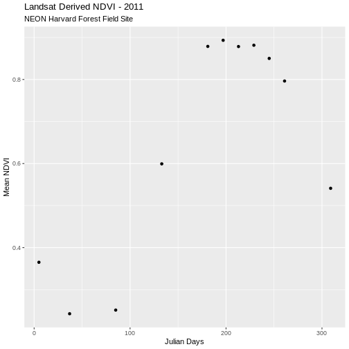
Now our outlier data points are removed and the pattern of “green-up” and “brown-down” makes more sense.
Write NDVI data to a .csv File
We can write our final NDVI dataframe out to a text format, to quickly share with a colleague or to reuse for analysis or visualization purposes. We will export in Comma Seperated Value (.csv) file format because it is usable in many different tools and across platforms (MAC, PC, etc).
We will use write.csv() to write a specified dataframe
to a .csv file. Unless you designate a different directory,
the output file will be saved in your working directory.
Before saving our file, let’s view the format to make sure it is what we want as an output format.
R
head(avg_NDVI_HARV_clean)
OUTPUT
meanNDVI site year julianDay Date
X005_HARV_ndvi_crop 0.365150 HARV 2011 5 2011-01-05
X037_HARV_ndvi_crop 0.242645 HARV 2011 37 2011-02-06
X085_HARV_ndvi_crop 0.251390 HARV 2011 85 2011-03-26
X133_HARV_ndvi_crop 0.599300 HARV 2011 133 2011-05-13
X181_HARV_ndvi_crop 0.878725 HARV 2011 181 2011-06-30
X197_HARV_ndvi_crop 0.893250 HARV 2011 197 2011-07-16It looks like we have a series of row.names that we do
not need because we have this information stored in individual columns
in our data frame. Let’s remove the row names.
R
row.names(avg_NDVI_HARV_clean) <- NULL
head(avg_NDVI_HARV_clean)
OUTPUT
meanNDVI site year julianDay Date
1 0.365150 HARV 2011 5 2011-01-05
2 0.242645 HARV 2011 37 2011-02-06
3 0.251390 HARV 2011 85 2011-03-26
4 0.599300 HARV 2011 133 2011-05-13
5 0.878725 HARV 2011 181 2011-06-30
6 0.893250 HARV 2011 197 2011-07-16R
write.csv(avg_NDVI_HARV_clean, file="meanNDVI_HARV_2011.csv")
Challenge: Write to .csv
- Create a NDVI .csv file for the NEON SJER field site that is comparable with the one we just created for the Harvard Forest. Be sure to inspect for questionable values before writing any data to a .csv file.
- Create a NDVI .csv file that includes data from both field sites.
R
avg_NDVI_SJER_clean <- subset(avg_NDVI_SJER, meanNDVI > 0.1)
row.names(avg_NDVI_SJER_clean) <- NULL
head(avg_NDVI_SJER_clean)
OUTPUT
meanNDVI site year julianDay Date
1 0.529780 SJER 2011 46 2011-02-15
2 0.554368 SJER 2011 62 2011-03-03
3 0.601096 SJER 2011 94 2011-04-04
4 0.555836 SJER 2011 110 2011-04-20
5 0.538336 SJER 2011 126 2011-05-06
6 0.400868 SJER 2011 142 2011-05-22R
write.csv(avg_NDVI_SJER_clean, file = "meanNDVI_SJER_2011.csv")
Key Points
- Use the
global()function to calculate summary statistics for cells in a raster object. - The pipe (
|) operator meansor. - Use the
rbind()function to combine data frames that have the same column names.