Work with Multi-Band Rasters
Last updated on 2025-05-13 | Edit this page
Overview
Questions
- How can I visualize individual and multiple bands in a raster object?
Objectives
- Identify a single vs. a multi-band raster file.
- Import multi-band rasters into R using the
terrapackage. - Plot multi-band color image rasters in R using the
ggplotpackage.
Things You’ll Need To Complete This Episode
See the lesson homepage for detailed information about the software, data, and other prerequisites you will need to work through the examples in this episode.
We introduced multi-band raster data in an earlier lesson. This episode explores how to import and plot a multi-band raster in R.
Getting Started with Multi-Band Data in R
In this episode, the multi-band data that we are working with is imagery collected using the NEON Airborne Observation Platform high resolution camera over the NEON Harvard Forest field site. Each RGB image is a 3-band raster. The same steps would apply to working with a multi-spectral image with 4 or more bands - like Landsat imagery.
By using the rast() function along with the
lyrs parameter, we can read specific raster bands (i.e. the
first one); omitting this parameter would read instead all bands.
R
RGB_band1_HARV <-
  rast("data/NEON-DS-Airborne-Remote-Sensing/HARV/RGB_Imagery/HARV_RGB_Ortho.tif",
       lyrs = 1)
We need to convert this data to a data frame in order to plot it with
ggplot.
R
RGB_band1_HARV_df <- as.data.frame(RGB_band1_HARV, xy = TRUE)R
ggplot() +
  geom_raster(data = RGB_band1_HARV_df,
              aes(x = x, y = y, alpha = HARV_RGB_Ortho_1)) +
  coord_quickmap()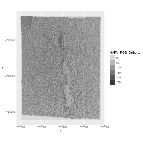
Challenge
View the attributes of this band. What are its dimensions, CRS, resolution, min and max values, and band number?
R
RGB_band1_HARVOUTPUT
class       : SpatRaster
dimensions  : 2317, 3073, 1  (nrow, ncol, nlyr)
resolution  : 0.25, 0.25  (x, y)
extent      : 731998.5, 732766.8, 4712956, 4713536  (xmin, xmax, ymin, ymax)
coord. ref. : WGS 84 / UTM zone 18N (EPSG:32618)
source      : HARV_RGB_Ortho.tif
name        : HARV_RGB_Ortho_1
min value   :                0
max value   :              255
Notice that when we look at the attributes of this band, we see:
dimensions : 2317, 3073, 1 (nrow, ncol, nlyr)
This is R telling us that we read only one its bands.
Data Tip
The number of bands associated with a raster’s file can also be
determined using the describe() function: syntax is
describe(sources(RGB_band1_HARV)).
Image Raster Data Values
As we saw in the previous exercise, this raster contains values between 0 and 255. These values represent degrees of brightness associated with the image band. In the case of a RGB image (red, green and blue), band 1 is the red band. When we plot the red band, larger numbers (towards 255) represent pixels with more red in them (a strong red reflection). Smaller numbers (towards 0) represent pixels with less red in them (less red was reflected). To plot an RGB image, we mix red + green + blue values into one single color to create a full color image - similar to the color image a digital camera creates.
Import A Specific Band
We can use the rast() function to import specific bands
in our raster object by specifying which band we want with
lyrs = N (N represents the band number we want to work
with). To import the green band, we would use lyrs = 2.
R
RGB_band2_HARV <-
  rast("data/NEON-DS-Airborne-Remote-Sensing/HARV/RGB_Imagery/HARV_RGB_Ortho.tif",
       lyrs = 2)
We can convert this data to a data frame and plot the same way we plotted the red band:
R
RGB_band2_HARV_df <- as.data.frame(RGB_band2_HARV, xy = TRUE)R
ggplot() +
  geom_raster(data = RGB_band2_HARV_df,
              aes(x = x, y = y, alpha = HARV_RGB_Ortho_2)) +
  coord_equal()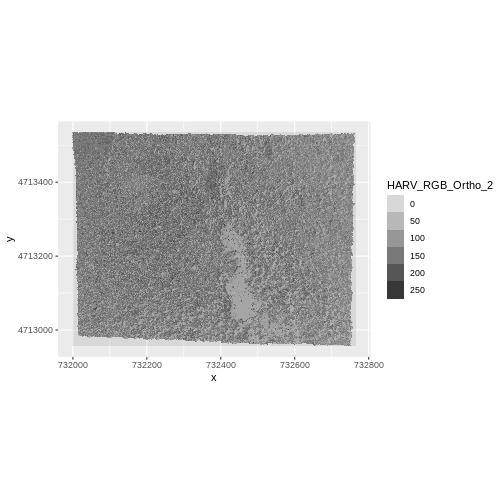
Challenge: Making Sense of Single Band Images
Compare the plots of band 1 (red) and band 2 (green). Is the forested area darker or lighter in band 2 (the green band) compared to band 1 (the red band)?
We’d expect a brighter value for the forest in band 2 (green) than in band 1 (red) because the leaves on trees of most often appear “green” - healthy leaves reflect MORE green light than red light.
Raster Stacks in R
Next, we will work with all three image bands (red, green and blue) as an R raster object. We will then plot a 3-band composite, or full color, image.
To bring in all bands of a multi-band raster, we use
therast() function.
R
RGB_stack_HARV <-
  rast("data/NEON-DS-Airborne-Remote-Sensing/HARV/RGB_Imagery/HARV_RGB_Ortho.tif")
Let’s preview the attributes of our stack object:
R
RGB_stack_HARVOUTPUT
class       : SpatRaster
dimensions  : 2317, 3073, 3  (nrow, ncol, nlyr)
resolution  : 0.25, 0.25  (x, y)
extent      : 731998.5, 732766.8, 4712956, 4713536  (xmin, xmax, ymin, ymax)
coord. ref. : WGS 84 / UTM zone 18N (EPSG:32618)
source      : HARV_RGB_Ortho.tif
names       : HARV_RGB_Ortho_1, HARV_RGB_Ortho_2, HARV_RGB_Ortho_3
min values  :                0,                0,                0
max values  :              255,              255,              255
We can view the attributes of each band in the stack in a single output. For example, if we had hundreds of bands, we could specify which band we’d like to view attributes for using an index value:
R
RGB_stack_HARV[[2]]OUTPUT
class       : SpatRaster
dimensions  : 2317, 3073, 1  (nrow, ncol, nlyr)
resolution  : 0.25, 0.25  (x, y)
extent      : 731998.5, 732766.8, 4712956, 4713536  (xmin, xmax, ymin, ymax)
coord. ref. : WGS 84 / UTM zone 18N (EPSG:32618)
source      : HARV_RGB_Ortho.tif
name        : HARV_RGB_Ortho_2
min value   :                0
max value   :              255
We can also use the ggplot functions to plot the data in
any layer of our raster object. Remember, we need to convert to a data
frame first.
R
RGB_stack_HARV_df <- as.data.frame(RGB_stack_HARV, xy = TRUE)Each band in our RasterStack gets its own column in the data frame. Thus we have:
R
str(RGB_stack_HARV_df)OUTPUT
'data.frame':	7120141 obs. of  5 variables:
 $ x               : num  731999 731999 731999 731999 732000 ...
 $ y               : num  4713535 4713535 4713535 4713535 4713535 ...
 $ HARV_RGB_Ortho_1: num  0 2 6 0 16 0 0 6 1 5 ...
 $ HARV_RGB_Ortho_2: num  1 0 9 0 5 0 4 2 1 0 ...
 $ HARV_RGB_Ortho_3: num  0 10 1 0 17 0 4 0 0 7 ...
Let’s create a histogram of the first band:
R
ggplot() +
  geom_histogram(data = RGB_stack_HARV_df, aes(HARV_RGB_Ortho_1))
OUTPUT
`stat_bin()` using `bins = 30`. Pick better value with `binwidth`.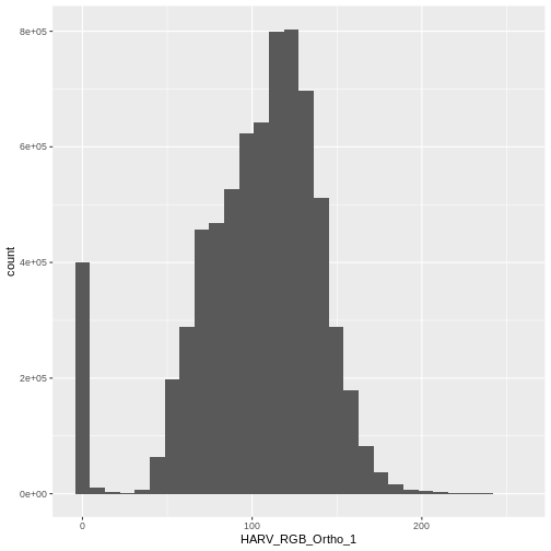
And a raster plot of the second band:
R
ggplot() +
  geom_raster(data = RGB_stack_HARV_df,
              aes(x = x, y = y, alpha = HARV_RGB_Ortho_2)) +
  coord_quickmap()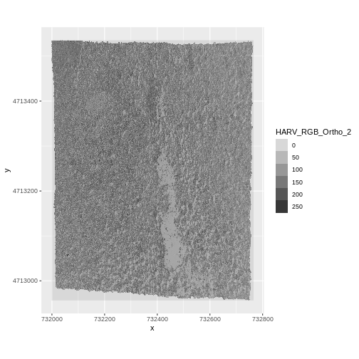
We can access any individual band in the same way.
Create A Three Band Image
To render a final three band, colored image in R, we use the
plotRGB() function.
This function allows us to:
- Identify what bands we want to render in the red, green and blue
regions. The
plotRGB()function defaults to a 1=red, 2=green, and 3=blue band order. However, you can define what bands you’d like to plot manually. Manual definition of bands is useful if you have, for example a near-infrared band and want to create a color infrared image. - Adjust the
stretchof the image to increase or decrease contrast.
Let’s plot our 3-band image. Note that we can use the
plotRGB() function directly with our RasterStack object (we
don’t need a dataframe as this function isn’t part of the
ggplot2 package).
R
plotRGB(RGB_stack_HARV,
        r = 1, g = 2, b = 3)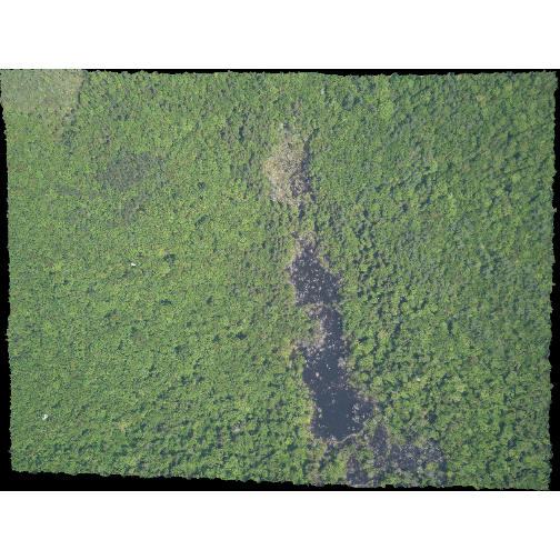
The image above looks pretty good. We can explore whether applying a
stretch to the image might improve clarity and contrast using
stretch="lin" or stretch="hist".
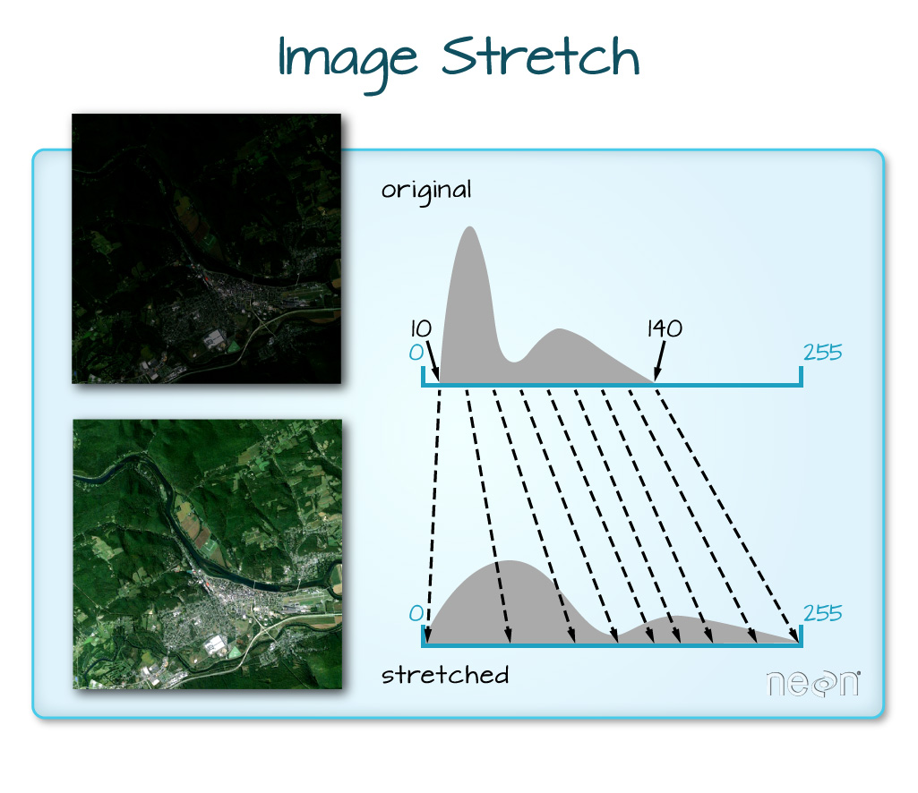
When the range of pixel brightness values is closer to 0, a darker image is rendered by default. We can stretch the values to extend to the full 0-255 range of potential values to increase the visual contrast of the image.
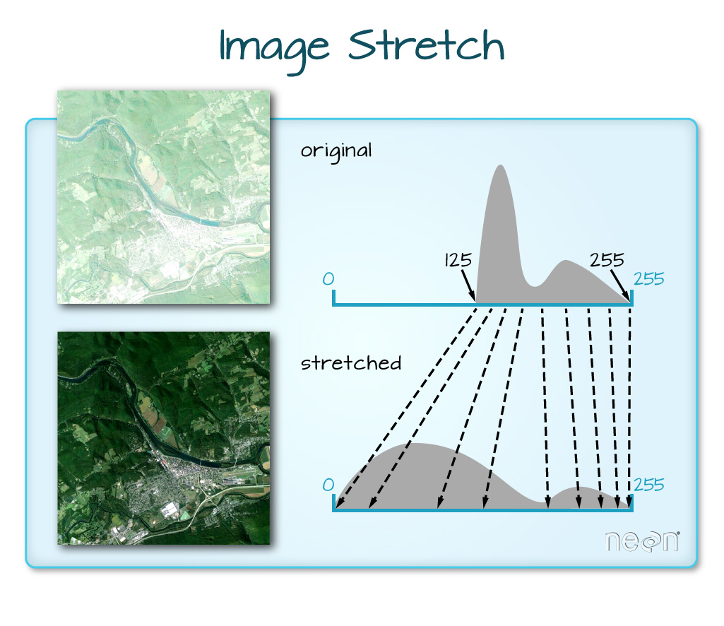
When the range of pixel brightness values is closer to 255, a lighter image is rendered by default. We can stretch the values to extend to the full 0-255 range of potential values to increase the visual contrast of the image.
R
plotRGB(RGB_stack_HARV,
        r = 1, g = 2, b = 3,
        scale = 800,
        stretch = "lin")
ERROR
Error in grDevices::rgb(RGB[, 1], RGB[, 2], RGB[, 3], alpha = alpha, maxColorValue = scale): alpha level 800, not in 0:255R
plotRGB(RGB_stack_HARV,
        r = 1, g = 2, b = 3,
        scale = 800,
        stretch = "hist")
ERROR
Error in grDevices::rgb(RGB[, 1], RGB[, 2], RGB[, 3], alpha = alpha, maxColorValue = scale): alpha level 800, not in 0:255In this case, the stretch doesn’t enhance the contrast our image significantly given the distribution of reflectance (or brightness) values is distributed well between 0 and 255.
Challenge - NoData Values
Let’s explore what happens with NoData values when working with
RasterStack objects and using the plotRGB() function. We
will use the HARV_Ortho_wNA.tif GeoTIFF file in the
NEON-DS-Airborne-Remote-Sensing/HARV/RGB_Imagery/
directory.
- View the files attributes. Are there
NoDatavalues assigned for this file? - If so, what is the
NoDataValue? - How many bands does it have?
- Load the multi-band raster file into R.
- Plot the object as a true color image.
- What happened to the black edges in the data?
- What does this tell us about the difference in the data structure
between
HARV_Ortho_wNA.tifandHARV_RGB_Ortho.tif(R objectRGB_stack). How can you check?
- First we use the
describe()function to view the data attributes.
R
describe("data/NEON-DS-Airborne-Remote-Sensing/HARV/RGB_Imagery/HARV_Ortho_wNA.tif")OUTPUT
 [1] "Driver: GTiff/GeoTIFF"
 [2] "Files: data/NEON-DS-Airborne-Remote-Sensing/HARV/RGB_Imagery/HARV_Ortho_wNA.tif"
 [3] "Size is 3073, 2317"
 [4] "Coordinate System is:"
 [5] "PROJCRS[\"WGS 84 / UTM zone 18N\","
 [6] "    BASEGEOGCRS[\"WGS 84\","
 [7] "        DATUM[\"World Geodetic System 1984\","
 [8] "            ELLIPSOID[\"WGS 84\",6378137,298.257223563,"
 [9] "                LENGTHUNIT[\"metre\",1]]],"
[10] "        PRIMEM[\"Greenwich\",0,"
[11] "            ANGLEUNIT[\"degree\",0.0174532925199433]],"
[12] "        ID[\"EPSG\",4326]],"
[13] "    CONVERSION[\"UTM zone 18N\","
[14] "        METHOD[\"Transverse Mercator\","
[15] "            ID[\"EPSG\",9807]],"
[16] "        PARAMETER[\"Latitude of natural origin\",0,"
[17] "            ANGLEUNIT[\"degree\",0.0174532925199433],"
[18] "            ID[\"EPSG\",8801]],"
[19] "        PARAMETER[\"Longitude of natural origin\",-75,"
[20] "            ANGLEUNIT[\"degree\",0.0174532925199433],"
[21] "            ID[\"EPSG\",8802]],"
[22] "        PARAMETER[\"Scale factor at natural origin\",0.9996,"
[23] "            SCALEUNIT[\"unity\",1],"
[24] "            ID[\"EPSG\",8805]],"
[25] "        PARAMETER[\"False easting\",500000,"
[26] "            LENGTHUNIT[\"metre\",1],"
[27] "            ID[\"EPSG\",8806]],"
[28] "        PARAMETER[\"False northing\",0,"
[29] "            LENGTHUNIT[\"metre\",1],"
[30] "            ID[\"EPSG\",8807]]],"
[31] "    CS[Cartesian,2],"
[32] "        AXIS[\"(E)\",east,"
[33] "            ORDER[1],"
[34] "            LENGTHUNIT[\"metre\",1]],"
[35] "        AXIS[\"(N)\",north,"
[36] "            ORDER[2],"
[37] "            LENGTHUNIT[\"metre\",1]],"
[38] "    USAGE["
[39] "        SCOPE[\"Engineering survey, topographic mapping.\"],"
[40] "        AREA[\"Between 78°W and 72°W, northern hemisphere between equator and 84°N, onshore and offshore. Bahamas. Canada - Nunavut; Ontario; Quebec. Colombia. Cuba. Ecuador. Greenland. Haiti. Jamica. Panama. Turks and Caicos Islands. United States (USA). Venezuela.\"],"
[41] "        BBOX[0,-78,84,-72]],"
[42] "    ID[\"EPSG\",32618]]"
[43] "Data axis to CRS axis mapping: 1,2"
[44] "Origin = (731998.500000000000000,4713535.500000000000000)"
[45] "Pixel Size = (0.250000000000000,-0.250000000000000)"
[46] "Metadata:"
[47] "  AREA_OR_POINT=Area"
[48] "Image Structure Metadata:"
[49] "  COMPRESSION=LZW"
[50] "  INTERLEAVE=PIXEL"
[51] "Corner Coordinates:"
[52] "Upper Left  (  731998.500, 4713535.500) ( 72d10'29.27\"W, 42d32'21.80\"N)"
[53] "Lower Left  (  731998.500, 4712956.250) ( 72d10'30.11\"W, 42d32' 3.04\"N)"
[54] "Upper Right (  732766.750, 4713535.500) ( 72d 9'55.63\"W, 42d32'20.97\"N)"
[55] "Lower Right (  732766.750, 4712956.250) ( 72d 9'56.48\"W, 42d32' 2.21\"N)"
[56] "Center      (  732382.625, 4713245.875) ( 72d10'12.87\"W, 42d32'12.00\"N)"
[57] "Band 1 Block=3073x1 Type=Float64, ColorInterp=Gray"
[58] "  Min=0.000 Max=255.000 "
[59] "  Minimum=0.000, Maximum=255.000, Mean=107.837, StdDev=30.019"
[60] "  NoData Value=-9999"
[61] "  Metadata:"
[62] "    STATISTICS_MAXIMUM=255"
[63] "    STATISTICS_MEAN=107.83651227531"
[64] "    STATISTICS_MINIMUM=0"
[65] "    STATISTICS_STDDEV=30.019177549096"
[66] "Band 2 Block=3073x1 Type=Float64, ColorInterp=Undefined"
[67] "  Min=0.000 Max=255.000 "
[68] "  Minimum=0.000, Maximum=255.000, Mean=130.096, StdDev=32.002"
[69] "  NoData Value=-9999"
[70] "  Metadata:"
[71] "    STATISTICS_MAXIMUM=255"
[72] "    STATISTICS_MEAN=130.09595363812"
[73] "    STATISTICS_MINIMUM=0"
[74] "    STATISTICS_STDDEV=32.001675868273"
[75] "Band 3 Block=3073x1 Type=Float64, ColorInterp=Undefined"
[76] "  Min=0.000 Max=255.000 "
[77] "  Minimum=0.000, Maximum=255.000, Mean=95.760, StdDev=16.577"
[78] "  NoData Value=-9999"
[79] "  Metadata:"
[80] "    STATISTICS_MAXIMUM=255"
[81] "    STATISTICS_MEAN=95.759787935476"
[82] "    STATISTICS_MINIMUM=0"
[83] "    STATISTICS_STDDEV=16.577042076977"
From the output above, we see that there are
NoDatavalues and they are assigned the value of -9999.The data has three bands.
To read in the file, we will use the
rast()function:
R
HARV_NA <-
rast("data/NEON-DS-Airborne-Remote-Sensing/HARV/RGB_Imagery/HARV_Ortho_wNA.tif")- We can plot the data with the
plotRGB()function:
R
plotRGB(HARV_NA,
        r = 1, g = 2, b = 3)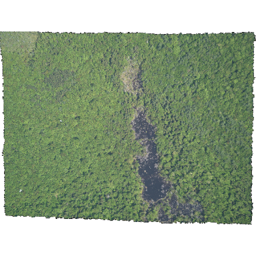
The black edges are not plotted.
Both data sets have
NoDatavalues, however, in the RGB_stack the NoData value is not defined in the tiff tags, thus R renders them as black as the reflectance values are 0. The black edges in the other file are defined as -9999 and R renders them as NA.
R
describe("data/NEON-DS-Airborne-Remote-Sensing/HARV/RGB_Imagery/HARV_RGB_Ortho.tif")OUTPUT
 [1] "Driver: GTiff/GeoTIFF"
 [2] "Files: data/NEON-DS-Airborne-Remote-Sensing/HARV/RGB_Imagery/HARV_RGB_Ortho.tif"
 [3] "Size is 3073, 2317"
 [4] "Coordinate System is:"
 [5] "PROJCRS[\"WGS 84 / UTM zone 18N\","
 [6] "    BASEGEOGCRS[\"WGS 84\","
 [7] "        DATUM[\"World Geodetic System 1984\","
 [8] "            ELLIPSOID[\"WGS 84\",6378137,298.257223563,"
 [9] "                LENGTHUNIT[\"metre\",1]]],"
[10] "        PRIMEM[\"Greenwich\",0,"
[11] "            ANGLEUNIT[\"degree\",0.0174532925199433]],"
[12] "        ID[\"EPSG\",4326]],"
[13] "    CONVERSION[\"UTM zone 18N\","
[14] "        METHOD[\"Transverse Mercator\","
[15] "            ID[\"EPSG\",9807]],"
[16] "        PARAMETER[\"Latitude of natural origin\",0,"
[17] "            ANGLEUNIT[\"degree\",0.0174532925199433],"
[18] "            ID[\"EPSG\",8801]],"
[19] "        PARAMETER[\"Longitude of natural origin\",-75,"
[20] "            ANGLEUNIT[\"degree\",0.0174532925199433],"
[21] "            ID[\"EPSG\",8802]],"
[22] "        PARAMETER[\"Scale factor at natural origin\",0.9996,"
[23] "            SCALEUNIT[\"unity\",1],"
[24] "            ID[\"EPSG\",8805]],"
[25] "        PARAMETER[\"False easting\",500000,"
[26] "            LENGTHUNIT[\"metre\",1],"
[27] "            ID[\"EPSG\",8806]],"
[28] "        PARAMETER[\"False northing\",0,"
[29] "            LENGTHUNIT[\"metre\",1],"
[30] "            ID[\"EPSG\",8807]]],"
[31] "    CS[Cartesian,2],"
[32] "        AXIS[\"(E)\",east,"
[33] "            ORDER[1],"
[34] "            LENGTHUNIT[\"metre\",1]],"
[35] "        AXIS[\"(N)\",north,"
[36] "            ORDER[2],"
[37] "            LENGTHUNIT[\"metre\",1]],"
[38] "    USAGE["
[39] "        SCOPE[\"Engineering survey, topographic mapping.\"],"
[40] "        AREA[\"Between 78°W and 72°W, northern hemisphere between equator and 84°N, onshore and offshore. Bahamas. Canada - Nunavut; Ontario; Quebec. Colombia. Cuba. Ecuador. Greenland. Haiti. Jamica. Panama. Turks and Caicos Islands. United States (USA). Venezuela.\"],"
[41] "        BBOX[0,-78,84,-72]],"
[42] "    ID[\"EPSG\",32618]]"
[43] "Data axis to CRS axis mapping: 1,2"
[44] "Origin = (731998.500000000000000,4713535.500000000000000)"
[45] "Pixel Size = (0.250000000000000,-0.250000000000000)"
[46] "Metadata:"
[47] "  AREA_OR_POINT=Area"
[48] "Image Structure Metadata:"
[49] "  COMPRESSION=LZW"
[50] "  INTERLEAVE=PIXEL"
[51] "Corner Coordinates:"
[52] "Upper Left  (  731998.500, 4713535.500) ( 72d10'29.27\"W, 42d32'21.80\"N)"
[53] "Lower Left  (  731998.500, 4712956.250) ( 72d10'30.11\"W, 42d32' 3.04\"N)"
[54] "Upper Right (  732766.750, 4713535.500) ( 72d 9'55.63\"W, 42d32'20.97\"N)"
[55] "Lower Right (  732766.750, 4712956.250) ( 72d 9'56.48\"W, 42d32' 2.21\"N)"
[56] "Center      (  732382.625, 4713245.875) ( 72d10'12.87\"W, 42d32'12.00\"N)"
[57] "Band 1 Block=3073x1 Type=Float64, ColorInterp=Gray"
[58] "  Min=0.000 Max=255.000 "
[59] "  Minimum=0.000, Maximum=255.000, Mean=nan, StdDev=nan"
[60] "  NoData Value=-1.69999999999999994e+308"
[61] "  Metadata:"
[62] "    STATISTICS_MAXIMUM=255"
[63] "    STATISTICS_MEAN=nan"
[64] "    STATISTICS_MINIMUM=0"
[65] "    STATISTICS_STDDEV=nan"
[66] "Band 2 Block=3073x1 Type=Float64, ColorInterp=Undefined"
[67] "  Min=0.000 Max=255.000 "
[68] "  Minimum=0.000, Maximum=255.000, Mean=nan, StdDev=nan"
[69] "  NoData Value=-1.69999999999999994e+308"
[70] "  Metadata:"
[71] "    STATISTICS_MAXIMUM=255"
[72] "    STATISTICS_MEAN=nan"
[73] "    STATISTICS_MINIMUM=0"
[74] "    STATISTICS_STDDEV=nan"
[75] "Band 3 Block=3073x1 Type=Float64, ColorInterp=Undefined"
[76] "  Min=0.000 Max=255.000 "
[77] "  Minimum=0.000, Maximum=255.000, Mean=nan, StdDev=nan"
[78] "  NoData Value=-1.69999999999999994e+308"
[79] "  Metadata:"
[80] "    STATISTICS_MAXIMUM=255"
[81] "    STATISTICS_MEAN=nan"
[82] "    STATISTICS_MINIMUM=0"
[83] "    STATISTICS_STDDEV=nan"
Data Tip
We can create a raster object from several, individual single-band GeoTIFFs too. We will do this in a later episode, Raster Time Series Data in R.
SpatRaster in R
The R SpatRaster object type can handle rasters with multiple bands. The SpatRaster only holds parameters that describe the properties of raster data that is located somewhere on our computer.
A SpatRasterDataset object can hold references to sub-datasets, that is, SpatRaster objects. In most cases, we can work with a SpatRaster in the same way we might work with a SpatRasterDataset.
More Resources
You can read the help for the rast() and
sds() functions by typing ?rast or
?sds.
We can build a SpatRasterDataset using a SpatRaster or a list of SpatRaster:
R
RGB_sds_HARV <- sds(RGB_stack_HARV)
RGB_sds_HARV <- sds(list(RGB_stack_HARV, RGB_stack_HARV))
We can retrieve the SpatRaster objects from a SpatRasterDataset using subsetting:
R
RGB_sds_HARV[[1]]OUTPUT
class       : SpatRaster
dimensions  : 2317, 3073, 3  (nrow, ncol, nlyr)
resolution  : 0.25, 0.25  (x, y)
extent      : 731998.5, 732766.8, 4712956, 4713536  (xmin, xmax, ymin, ymax)
coord. ref. : WGS 84 / UTM zone 18N (EPSG:32618)
source      : HARV_RGB_Ortho.tif
names       : HARV_RGB_Ortho_1, HARV_RGB_Ortho_2, HARV_RGB_Ortho_3
min values  :                0,                0,                0
max values  :              255,              255,              255
R
RGB_sds_HARV[[2]]OUTPUT
class       : SpatRaster
dimensions  : 2317, 3073, 3  (nrow, ncol, nlyr)
resolution  : 0.25, 0.25  (x, y)
extent      : 731998.5, 732766.8, 4712956, 4713536  (xmin, xmax, ymin, ymax)
coord. ref. : WGS 84 / UTM zone 18N (EPSG:32618)
source      : HARV_RGB_Ortho.tif
names       : HARV_RGB_Ortho_1, HARV_RGB_Ortho_2, HARV_RGB_Ortho_3
min values  :                0,                0,                0
max values  :              255,              255,              255
Challenge: What Functions Can Be Used on an R Object of a particular class?
We can view various functions (or methods) available to use on an R
object with methods(class=class(objectNameHere)). Use this
to figure out:
- What methods can be used on the
RGB_stack_HARVobject? - What methods can be used on a single band within
RGB_stack_HARV? - Why do you think there isn’t a difference?
- We can see a list of all of the methods available for our RasterStack object:
R
methods(class=class(RGB_stack_HARV))OUTPUT
  [1] !                     [                     [[
  [4] [[<-                  [<-                   %in%
  [7] $                     $<-                   activeCat
 [10] activeCat<-           add<-                 addCats
 [13] adjacent              aggregate             align
 [16] all.equal             allNA                 animate
 [19] anyNA                 app                   approximate
 [22] area                  Arith                 as.array
 [25] as.bool               as.character          as.contour
 [28] as.data.frame         as.factor             as.int
 [31] as.integer            as.lines              as.list
 [34] as.logical            as.matrix             as.numeric
 [37] as.points             as.polygons           as.raster
 [40] atan_2                atan2                 autocor
 [43] barplot               bestMatch             blocks
 [46] boundaries            boxplot               buffer
 [49] c                     catalyze              categories
 [52] cats                  cellFromRowCol        cellFromRowColCombine
 [55] cellFromXY            cells                 cellSize
 [58] clamp_ts              clamp                 classify
 [61] click                 coerce                colFromCell
 [64] colFromX              colMeans              colorize
 [67] colSums               coltab                coltab<-
 [70] Compare               compare               compareGeom
 [73] concats               contour               costDist
 [76] countNA               cover                 crds
 [79] crop                  crosstab              crs
 [82] crs<-                 datatype              deepcopy
 [85] density               depth                 depth<-
 [88] depthName             depthName<-           depthUnit
 [91] depthUnit<-           describe              diff
 [94] dim                   dim<-                 direction
 [97] disagg                distance              divide
[100] droplevels            expanse               ext
[103] ext<-                 extend                extract
[106] extractRange          fillTime              flip
[109] flowAccumulation      focal                 focal3D
[112] focalCpp              focalPairs            focalReg
[115] focalValues           freq                  getTileExtents
[118] global                gridDist              gridDistance
[121] has.colors            has.RGB               has.time
[124] hasMinMax             hasValues             head
[127] hist                  identical             ifel
[130] image                 init                  inMemory
[133] inset                 interpIDW             interpNear
[136] interpolate           intersect             is.bool
[139] is.factor             is.finite             is.flipped
[142] is.infinite           is.int                is.lonlat
[145] is.na                 is.nan                is.num
[148] is.related            is.rotated            isFALSE
[151] isTRUE                k_means               lapp
[154] layerCor              levels                levels<-
[157] linearUnits           lines                 log
[160] Logic                 logic                 longnames
[163] longnames<-           makeTiles             mask
[166] match                 math                  Math
[169] Math2                 mean                  median
[172] merge                 meta                  metags
[175] metags<-              minmax                modal
[178] mosaic                NAflag                NAflag<-
[181] names                 names<-               ncell
[184] ncol                  ncol<-                NIDP
[187] nlyr                  nlyr<-                noNA
[190] not.na                nrow                  nrow<-
[193] nsrc                  origin                origin<-
[196] pairs                 panel                 patches
[199] persp                 pitfinder             plet
[202] plot                  plotRGB               points
[205] polys                 prcomp                predict
[208] princomp              project               quantile
[211] rangeFill             rapp                  rast
[214] rasterize             rasterizeGeom         rasterizeWin
[217] rcl                   readStart             readStop
[220] readValues            rectify               regress
[223] relate                rep                   res
[226] res<-                 resample              rescale
[229] rev                   RGB                   RGB<-
[232] roll                  rotate                rowColCombine
[235] rowColFromCell        rowFromCell           rowFromY
[238] rowMeans              rowSums               sapp
[241] saveRDS               scale_linear          scale
[244] scoff                 scoff<-               sds
[247] segregate             sel                   selectHighest
[250] selectRange           serialize             set.cats
[253] set.crs               set.ext               set.names
[256] set.RGB               set.values            set.window
[259] setMinMax             setValues             shift
[262] show                  sieve                 simplifyLevels
[265] size                  sort                  sources
[268] spatSample            split                 sprc
[271] stdev                 str                   stretch
[274] subset                subst                 summary
[277] Summary               surfArea              t
[280] tail                  tapp                  terrain
[283] text                  thresh                tighten
[286] time                  time<-                timeInfo
[289] toMemory              trans                 trim
[292] unique                units                 units<-
[295] update                values                values<-
[298] varnames              varnames<-            viewshed
[301] watershed             weighted.mean         where.max
[304] where.min             which.lyr             which.max
[307] which.min             window                window<-
[310] wrap                  wrapCache             writeCDF
[313] writeRaster           writeStart            writeStop
[316] writeValues           xapp                  xFromCell
[319] xFromCol              xmax                  xmax<-
[322] xmin                  xmin<-                xres
[325] xyFromCell            yFromCell             yFromRow
[328] ymax                  ymax<-                ymin
[331] ymin<-                yres                  zonal
[334] zoom
see '?methods' for accessing help and source code- And compare that with the methods available for a single band:
R
methods(class=class(RGB_stack_HARV[[1]]))OUTPUT
  [1] !                     [                     [[
  [4] [[<-                  [<-                   %in%
  [7] $                     $<-                   activeCat
 [10] activeCat<-           add<-                 addCats
 [13] adjacent              aggregate             align
 [16] all.equal             allNA                 animate
 [19] anyNA                 app                   approximate
 [22] area                  Arith                 as.array
 [25] as.bool               as.character          as.contour
 [28] as.data.frame         as.factor             as.int
 [31] as.integer            as.lines              as.list
 [34] as.logical            as.matrix             as.numeric
 [37] as.points             as.polygons           as.raster
 [40] atan_2                atan2                 autocor
 [43] barplot               bestMatch             blocks
 [46] boundaries            boxplot               buffer
 [49] c                     catalyze              categories
 [52] cats                  cellFromRowCol        cellFromRowColCombine
 [55] cellFromXY            cells                 cellSize
 [58] clamp_ts              clamp                 classify
 [61] click                 coerce                colFromCell
 [64] colFromX              colMeans              colorize
 [67] colSums               coltab                coltab<-
 [70] Compare               compare               compareGeom
 [73] concats               contour               costDist
 [76] countNA               cover                 crds
 [79] crop                  crosstab              crs
 [82] crs<-                 datatype              deepcopy
 [85] density               depth                 depth<-
 [88] depthName             depthName<-           depthUnit
 [91] depthUnit<-           describe              diff
 [94] dim                   dim<-                 direction
 [97] disagg                distance              divide
[100] droplevels            expanse               ext
[103] ext<-                 extend                extract
[106] extractRange          fillTime              flip
[109] flowAccumulation      focal                 focal3D
[112] focalCpp              focalPairs            focalReg
[115] focalValues           freq                  getTileExtents
[118] global                gridDist              gridDistance
[121] has.colors            has.RGB               has.time
[124] hasMinMax             hasValues             head
[127] hist                  identical             ifel
[130] image                 init                  inMemory
[133] inset                 interpIDW             interpNear
[136] interpolate           intersect             is.bool
[139] is.factor             is.finite             is.flipped
[142] is.infinite           is.int                is.lonlat
[145] is.na                 is.nan                is.num
[148] is.related            is.rotated            isFALSE
[151] isTRUE                k_means               lapp
[154] layerCor              levels                levels<-
[157] linearUnits           lines                 log
[160] Logic                 logic                 longnames
[163] longnames<-           makeTiles             mask
[166] match                 math                  Math
[169] Math2                 mean                  median
[172] merge                 meta                  metags
[175] metags<-              minmax                modal
[178] mosaic                NAflag                NAflag<-
[181] names                 names<-               ncell
[184] ncol                  ncol<-                NIDP
[187] nlyr                  nlyr<-                noNA
[190] not.na                nrow                  nrow<-
[193] nsrc                  origin                origin<-
[196] pairs                 panel                 patches
[199] persp                 pitfinder             plet
[202] plot                  plotRGB               points
[205] polys                 prcomp                predict
[208] princomp              project               quantile
[211] rangeFill             rapp                  rast
[214] rasterize             rasterizeGeom         rasterizeWin
[217] rcl                   readStart             readStop
[220] readValues            rectify               regress
[223] relate                rep                   res
[226] res<-                 resample              rescale
[229] rev                   RGB                   RGB<-
[232] roll                  rotate                rowColCombine
[235] rowColFromCell        rowFromCell           rowFromY
[238] rowMeans              rowSums               sapp
[241] saveRDS               scale_linear          scale
[244] scoff                 scoff<-               sds
[247] segregate             sel                   selectHighest
[250] selectRange           serialize             set.cats
[253] set.crs               set.ext               set.names
[256] set.RGB               set.values            set.window
[259] setMinMax             setValues             shift
[262] show                  sieve                 simplifyLevels
[265] size                  sort                  sources
[268] spatSample            split                 sprc
[271] stdev                 str                   stretch
[274] subset                subst                 summary
[277] Summary               surfArea              t
[280] tail                  tapp                  terrain
[283] text                  thresh                tighten
[286] time                  time<-                timeInfo
[289] toMemory              trans                 trim
[292] unique                units                 units<-
[295] update                values                values<-
[298] varnames              varnames<-            viewshed
[301] watershed             weighted.mean         where.max
[304] where.min             which.lyr             which.max
[307] which.min             window                window<-
[310] wrap                  wrapCache             writeCDF
[313] writeRaster           writeStart            writeStop
[316] writeValues           xapp                  xFromCell
[319] xFromCol              xmax                  xmax<-
[322] xmin                  xmin<-                xres
[325] xyFromCell            yFromCell             yFromRow
[328] ymax                  ymax<-                ymin
[331] ymin<-                yres                  zonal
[334] zoom
see '?methods' for accessing help and source code- A SpatRaster is the same no matter its number of bands.
Key Points
- A single raster file can contain multiple bands or layers.
- Use the
rast()function to load all bands in a multi-layer raster file into R. - Individual bands within a SpatRaster can be accessed, analyzed, and visualized using the same functions no matter how many bands it holds.