Explore and Plot by Vector Layer Attributes
Last updated on 2024-10-15 | Edit this page
Overview
Questions
- How can I compute on the attributes of a spatial object?
Objectives
- Query attributes of a spatial object.
- Subset spatial objects using specific attribute values.
- Plot a vector feature, colored by unique attribute values.
Things You’ll Need To Complete This Episode
See the lesson homepage for detailed information about the software, data, and other prerequisites you will need to work through the examples in this episode.
This episode continues our discussion of vector layer attributes and covers how to work with vector layer attributes in R. It covers how to identify and query layer attributes, as well as how to subset features by specific attribute values. Finally, we will learn how to plot a feature according to a set of attribute values.
Load the Data
We will continue using the sf, terra and
ggplot2 packages in this episode. Make sure that you have
these packages loaded. We will continue to work with the three ESRI
shapefiles (vector layers) that we loaded in the Open and Plot Vector Layers in
R episode.
Query Vector Feature Metadata
As we discussed in the Open and Plot Vector Layers in R episode, we can view metadata associated with an R object using:
-
st_geometry_type()- The type of vector data stored in the object. -
nrow()- The number of features in the object -
st_bbox()- The spatial extent (geographic area covered by) of the object. -
st_crs()- The CRS (spatial projection) of the data.
We started to explore our point_HARV object in the
previous episode. To see a summary of all of the metadata associated
with our point_HARV object, we can view the object with
View(point_HARV) or print a summary of the object itself to
the console.
R
point_HARV
OUTPUT
Simple feature collection with 1 feature and 14 fields
Geometry type: POINT
Dimension:     XY
Bounding box:  xmin: 732183.2 ymin: 4713265 xmax: 732183.2 ymax: 4713265
Projected CRS: WGS 84 / UTM zone 18N
  Un_ID Domain DomainName       SiteName Type       Sub_Type     Lat      Long
1     A      1  Northeast Harvard Forest Core Advanced Tower 42.5369 -72.17266
  Zone  Easting Northing                Ownership    County annotation
1   18 732183.2  4713265 Harvard University, LTER Worcester         C1
                  geometry
1 POINT (732183.2 4713265)
We can use the ncol function to count the number of
attributes associated with a spatial object too. Note that the geometry
is just another column and counts towards the total.
R
ncol(lines_HARV)
OUTPUT
[1] 16We can view the individual name of each attribute using the
names() function in R:
R
names(lines_HARV)
OUTPUT
 [1] "OBJECTID_1" "OBJECTID"   "TYPE"       "NOTES"      "MISCNOTES"
 [6] "RULEID"     "MAPLABEL"   "SHAPE_LENG" "LABEL"      "BIKEHORSE"
[11] "RESVEHICLE" "RECMAP"     "Shape_Le_1" "ResVehic_1" "BicyclesHo"
[16] "geometry"
We could also view just the first 6 rows of attribute values using
the head() function to get a preview of the data:
R
head(lines_HARV)
OUTPUT
Simple feature collection with 6 features and 15 fields
Geometry type: MULTILINESTRING
Dimension:     XY
Bounding box:  xmin: 730741.2 ymin: 4712685 xmax: 732232.3 ymax: 4713726
Projected CRS: WGS 84 / UTM zone 18N
  OBJECTID_1 OBJECTID       TYPE             NOTES MISCNOTES RULEID
1         14       48 woods road Locust Opening Rd      <NA>      5
2         40       91   footpath              <NA>      <NA>      6
3         41      106   footpath              <NA>      <NA>      6
4        211      279 stone wall              <NA>      <NA>      1
5        212      280 stone wall              <NA>      <NA>      1
6        213      281 stone wall              <NA>      <NA>      1
           MAPLABEL SHAPE_LENG             LABEL BIKEHORSE RESVEHICLE RECMAP
1 Locust Opening Rd 1297.35706 Locust Opening Rd         Y         R1      Y
2              <NA>  146.29984              <NA>         Y         R1      Y
3              <NA>  676.71804              <NA>         Y         R2      Y
4              <NA>  231.78957              <NA>      <NA>       <NA>   <NA>
5              <NA>   45.50864              <NA>      <NA>       <NA>   <NA>
6              <NA>  198.39043              <NA>      <NA>       <NA>   <NA>
  Shape_Le_1                            ResVehic_1                  BicyclesHo
1 1297.10617    R1 - All Research Vehicles Allowed Bicycles and Horses Allowed
2  146.29983    R1 - All Research Vehicles Allowed Bicycles and Horses Allowed
3  676.71807 R2 - 4WD/High Clearance Vehicles Only Bicycles and Horses Allowed
4  231.78962                                  <NA>                        <NA>
5   45.50859                                  <NA>                        <NA>
6  198.39041                                  <NA>                        <NA>
                        geometry
1 MULTILINESTRING ((730819.2 ...
2 MULTILINESTRING ((732040.2 ...
3 MULTILINESTRING ((732057 47...
4 MULTILINESTRING ((731903.6 ...
5 MULTILINESTRING ((732039.1 ...
6 MULTILINESTRING ((732056.2 ...
Challenge: Attributes for Different Spatial Classes
Explore the attributes associated with the point_HARV
and aoi_boundary_HARV spatial objects.
How many attributes does each have?
Who owns the site in the
point_HARVdata object?Which of the following is NOT an attribute of the
point_HARVdata object?
- Latitude B) County C) Country
- To find the number of attributes, we use the
ncol()function:
R
ncol(point_HARV)
OUTPUT
[1] 15R
ncol(aoi_boundary_HARV)
OUTPUT
[1] 2- Ownership information is in a column named
Ownership:
R
point_HARV$Ownership
OUTPUT
[1] "Harvard University, LTER"- To see a list of all of the attributes, we can use the
names()function:
R
names(point_HARV)
OUTPUT
 [1] "Un_ID"      "Domain"     "DomainName" "SiteName"   "Type"
 [6] "Sub_Type"   "Lat"        "Long"       "Zone"       "Easting"
[11] "Northing"   "Ownership"  "County"     "annotation" "geometry"
“Country” is not an attribute of this object.
Explore Values within One Attribute
We can explore individual values stored within a particular
attribute. Comparing attributes to a spreadsheet or a data frame, this
is similar to exploring values in a column. We did this with the
gapminder dataframe in an
earlier lesson. For spatial objects, we can use the same syntax:
objectName$attributeName.
We can see the contents of the TYPE field of our lines
feature:
R
lines_HARV$TYPE
OUTPUT
 [1] "woods road" "footpath"   "footpath"   "stone wall" "stone wall"
 [6] "stone wall" "stone wall" "stone wall" "stone wall" "boardwalk"
[11] "woods road" "woods road" "woods road"
To see only unique values within the TYPE field, we can
use the unique() function for extracting the possible
values of a character variable (R also is able to handle categorical
variables called factors; we worked with factors a little bit in an
earlier lesson.
R
unique(lines_HARV$TYPE)
OUTPUT
[1] "woods road" "footpath" "stone wall" "boardwalk" Subset Features
We can use the filter() function from dplyr
that we worked with in an earlier
lesson to select a subset of features from a spatial object in R,
just like with data frames.
For example, we might be interested only in features that are of
TYPE “footpath”. Once we subset out this data, we can use
it as input to other code so that code only operates on the footpath
lines.
R
footpath_HARV <- lines_HARV %>%
  filter(TYPE == "footpath")
nrow(footpath_HARV)
OUTPUT
[1] 2Our subsetting operation reduces the features count to
2. This means that only two feature lines in our spatial object have the
attribute TYPE == footpath. We can plot only the footpath
lines:
R
ggplot() +
  geom_sf(data = footpath_HARV) +
  ggtitle("NEON Harvard Forest Field Site", subtitle = "Footpaths") +
  coord_sf()
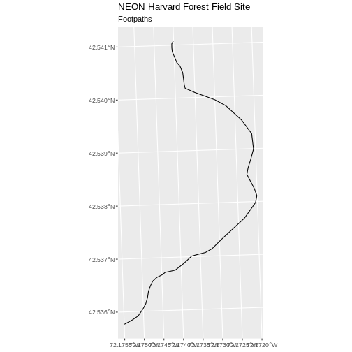
There are two features in our footpaths subset. Why does the plot
look like there is only one feature? Let’s adjust the colors used in our
plot. If we have 2 features in our vector object, we can plot each using
a unique color by assigning a column name to the color aesthetic
(color =). We use the syntax aes(color = ) to
do this. We can also alter the default line thickness by using the
size = parameter, as the default value of 0.5 can be hard
to see. Note that size is placed outside of the aes()
function, as we are not connecting line thickness to a data
variable.
R
ggplot() +
  geom_sf(data = footpath_HARV, aes(color = factor(OBJECTID)), size = 1.5) +
  labs(color = 'Footpath ID') +
  ggtitle("NEON Harvard Forest Field Site", subtitle = "Footpaths") +
  coord_sf()
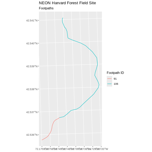
Now, we see that there are in fact two features in our plot!
Challenge: Subset Spatial Line Objects Part 1
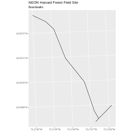
Subset out all boardwalk from the lines layer and plot
it.
First we will save an object with only the boardwalk lines:
R
boardwalk_HARV <- lines_HARV %>%
  filter(TYPE == "boardwalk")
Let’s check how many features there are in this subset:
R
nrow(boardwalk_HARV)
OUTPUT
[1] 1Now let’s plot that data:
R
ggplot() +
  geom_sf(data = boardwalk_HARV, size = 1.5) +
  ggtitle("NEON Harvard Forest Field Site", subtitle = "Boardwalks") +
  coord_sf()
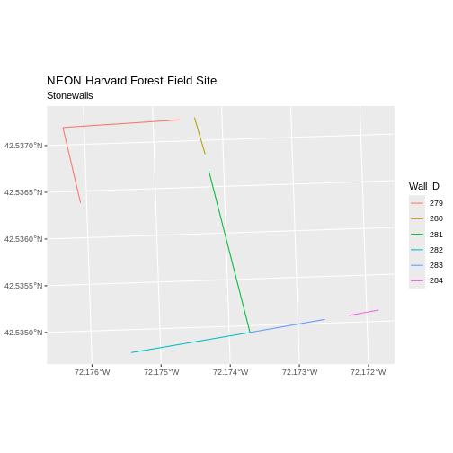
Challenge: Subset Spatial Line Objects Part 2
Subset out all stone wall features from the lines layer
and plot it. For each plot, color each feature using a unique color.
First we will save an object with only the stone wall lines and check the number of features:
R
stoneWall_HARV <- lines_HARV %>%
  filter(TYPE == "stone wall")
nrow(stoneWall_HARV)
OUTPUT
[1] 6Now we can plot the data:
R
ggplot() +
  geom_sf(data = stoneWall_HARV, aes(color = factor(OBJECTID)), size = 1.5) +
  labs(color = 'Wall ID') +
  ggtitle("NEON Harvard Forest Field Site", subtitle = "Stonewalls") +
  coord_sf()
Customize Plots
In the examples above, ggplot() automatically selected
colors for each line based on a default color order. If we don’t like
those default colors, we can create a vector of colors - one for each
feature.
First we will check how many unique levels our factor has:
R
unique(lines_HARV$TYPE)
OUTPUT
[1] "woods road" "footpath" "stone wall" "boardwalk" Then we can create a palette of four colors, one for each feature in our vector object.
R
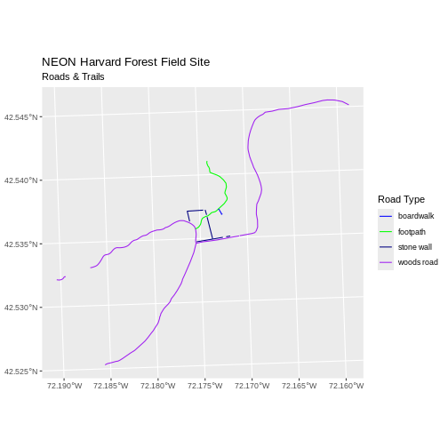
road_colors <- c("blue", "green", "navy", "purple")
We can tell ggplot to use these colors when we plot the
data.
R
ggplot() +
  geom_sf(data = lines_HARV, aes(color = TYPE)) +
  scale_color_manual(values = road_colors) +
  labs(color = 'Road Type') +
  ggtitle("NEON Harvard Forest Field Site", subtitle = "Roads & Trails") +
  coord_sf()
Adjust Line Width
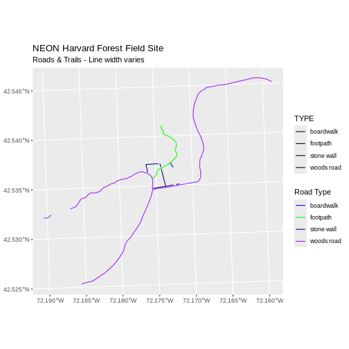
We adjusted line width universally earlier. If we want a unique line width for each level or attribute category in our spatial object, we can use the same syntax that we used for colors, above.
We already know that we have four different TYPEs in the
lines_HARV object, so we will set four different line widths.
R
line_widths <- c(1, 2, 3, 4)
We can use those line widths when we plot the data.
R
ggplot() +
  geom_sf(data = lines_HARV, aes(color = TYPE, size = TYPE)) +
  scale_color_manual(values = road_colors) +
  labs(color = 'Road Type') +
  scale_size_manual(values = line_widths) +
  ggtitle("NEON Harvard Forest Field Site",
          subtitle = "Roads & Trails - Line width varies") +
  coord_sf()
Challenge: Plot Line Width by Attribute
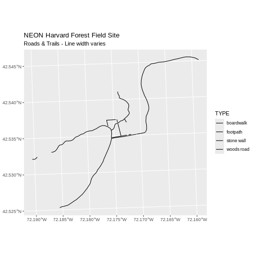
In the example above, we set the line widths to be 1, 2, 3, and 4. Because R orders alphabetically by default, this gave us a plot where woods roads (the last type) were the thickest and boardwalks were the thinnest.
Let’s create another plot where we show the different line types with the following thicknesses:
- woods road size = 6
- boardwalks size = 1
- footpath size = 3
- stone wall size = 2
First we need to look at the levels of our factor to see what order the road types are in:
R
unique(lines_HARV$TYPE)
OUTPUT
[1] "woods road" "footpath" "stone wall" "boardwalk" We then can create our line_width vector setting each of
the levels to the desired thickness.
R
line_width <- c(1, 3, 2, 6)
Now we can create our plot.
R
ggplot() +
  geom_sf(data = lines_HARV, aes(size = TYPE)) +
  scale_size_manual(values = line_width) +
  ggtitle("NEON Harvard Forest Field Site",
          subtitle = "Roads & Trails - Line width varies") +
  coord_sf()
Add Plot Legend
We can add a legend to our plot too. When we add a legend, we use the following elements to specify labels and colors:
-
bottomright: We specify the location of our legend by using a default keyword. We could also usetop,topright, etc. -
levels(objectName$attributeName): Label the legend elements using the categories of levels in an attribute (e.g., levels(lines_HARV$TYPE) means use the levels boardwalk, footpath, etc). -
fill =: apply unique colors to the boxes in our legend.palette()is the default set of colors that R applies to all plots.
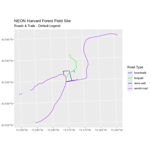
Let’s add a legend to our plot. We will use the
road_colors object that we created above to color the
legend. We can customize the appearance of our legend by manually
setting different parameters.
R
ggplot() +
  geom_sf(data = lines_HARV, aes(color = TYPE), size = 1.5) +
  scale_color_manual(values = road_colors) +
  labs(color = 'Road Type') +
  ggtitle("NEON Harvard Forest Field Site",
          subtitle = "Roads & Trails - Default Legend") +
  coord_sf()
We can change the appearance of our legend by manually setting different parameters.
-
legend.text: change the font size -
legend.box.background: add an outline box
R
ggplot() +
  geom_sf(data = lines_HARV, aes(color = TYPE), size = 1.5) +
  scale_color_manual(values = road_colors) +
  labs(color = 'Road Type') +
  theme(legend.text = element_text(size = 20),
        legend.box.background = element_rect(size = 1)) +
  ggtitle("NEON Harvard Forest Field Site",
          subtitle = "Roads & Trails - Modified Legend") +
  coord_sf()
WARNING
Warning: The `size` argument of `element_rect()` is deprecated as of ggplot2 3.4.0.
ℹ Please use the `linewidth` argument instead.
This warning is displayed once every 8 hours.
Call `lifecycle::last_lifecycle_warnings()` to see where this warning was
generated.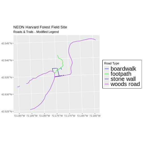
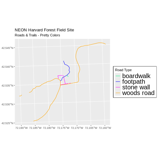
R
new_colors <- c("springgreen", "blue", "magenta", "orange")

ggplot() +
  geom_sf(data = lines_HARV, aes(color = TYPE), size = 1.5) +
  scale_color_manual(values = new_colors) +
  labs(color = 'Road Type') +
  theme(legend.text = element_text(size = 20),
        legend.box.background = element_rect(size = 1)) +
  ggtitle("NEON Harvard Forest Field Site",
          subtitle = "Roads & Trails - Pretty Colors") +
  coord_sf()
Data Tip
You can modify the default R color palette using the palette method.
For example palette(rainbow(6)) or
palette(terrain.colors(6)). You can reset the palette
colors using palette("default")!
You can also use colorblind-friendly palettes such as those in the viridis package.
Challenge: Plot Lines by Attribute
Create a plot that emphasizes only roads where bicycles and horses
are allowed. To emphasize this, make the lines where bicycles are not
allowed THINNER than the roads where bicycles are allowed. NOTE: this
attribute information is located in the
lines_HARV$BicyclesHo attribute.
Be sure to add a title and legend to your map. You might consider a color palette that has all bike/horse-friendly roads displayed in a bright color. All other lines can be black.
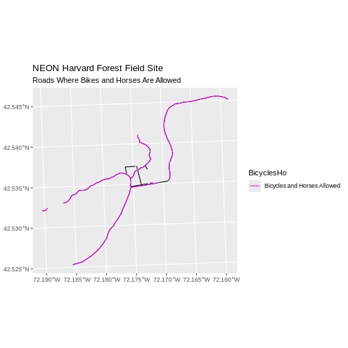
First we explore the BicyclesHo attribute to learn the
values that correspond to the roads we need.
R
lines_HARV %>%
  pull(BicyclesHo) %>%
  unique()
OUTPUT
[1] "Bicycles and Horses Allowed"     NA
[3] "DO NOT SHOW ON REC MAP"          "Bicycles and Horses NOT ALLOWED"
Now, we can create a data frame with only those roads where bicycles and horses are allowed.
R
lines_showHarv <-
  lines_HARV %>%
  filter(BicyclesHo == "Bicycles and Horses Allowed")
Finally, we plot the needed roads after setting them to magenta and a thicker line width.
R
ggplot() +
  geom_sf(data = lines_HARV) +
  geom_sf(data = lines_showHarv, aes(color = BicyclesHo), size = 2) +
  scale_color_manual(values = "magenta") +
  ggtitle("NEON Harvard Forest Field Site",
          subtitle = "Roads Where Bikes and Horses Are Allowed") +
  coord_sf()
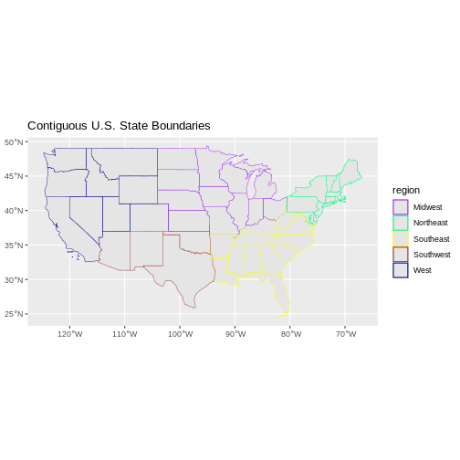
Challenge: Plot Polygon by Attribute
- Create a map of the state boundaries in the United States using the
data located in your downloaded data folder:
NEON-DS-Site-Layout-Files/US-Boundary-Layers\US-State-Boundaries-Census-2014. Apply a line color to each state using itsregionvalue. Add a legend.
First we read in the data and check how many levels there are in the
region column:
R
state_boundary_US <-
st_read("data/NEON-DS-Site-Layout-Files/US-Boundary-Layers/US-State-Boundaries-Census-2014.shp") %>%
# NOTE: We need neither Z nor M coordinates!
st_zm()
OUTPUT
Reading layer `US-State-Boundaries-Census-2014' from data source
  `/home/runner/work/r-raster-vector-geospatial/r-raster-vector-geospatial/site/built/data/NEON-DS-Site-Layout-Files/US-Boundary-Layers/US-State-Boundaries-Census-2014.shp'
  using driver `ESRI Shapefile'
Simple feature collection with 58 features and 10 fields
Geometry type: MULTIPOLYGON
Dimension:     XYZ
Bounding box:  xmin: -124.7258 ymin: 24.49813 xmax: -66.9499 ymax: 49.38436
z_range:       zmin: 0 zmax: 0
Geodetic CRS:  WGS 84
R
state_boundary_US$region <- as.factor(state_boundary_US$region)
levels(state_boundary_US$region)
OUTPUT
[1] "Midwest" "Northeast" "Southeast" "Southwest" "West" Next we set a color vector with that many items:
R
colors <- c("purple", "springgreen", "yellow", "brown", "navy")
Now we can create our plot:
R
ggplot() +
  geom_sf(data = state_boundary_US, aes(color = region), size = 1) +
  scale_color_manual(values = colors) +
  ggtitle("Contiguous U.S. State Boundaries") +
  coord_sf()
Key Points
- Spatial objects in
sfare similar to standard data frames and can be manipulated using the same functions. - Almost any feature of a plot can be customized using the various
functions and options in the
ggplot2package.