Open and Plot Vector Layers
Last updated on 2024-10-15 | Edit this page
Overview
Questions
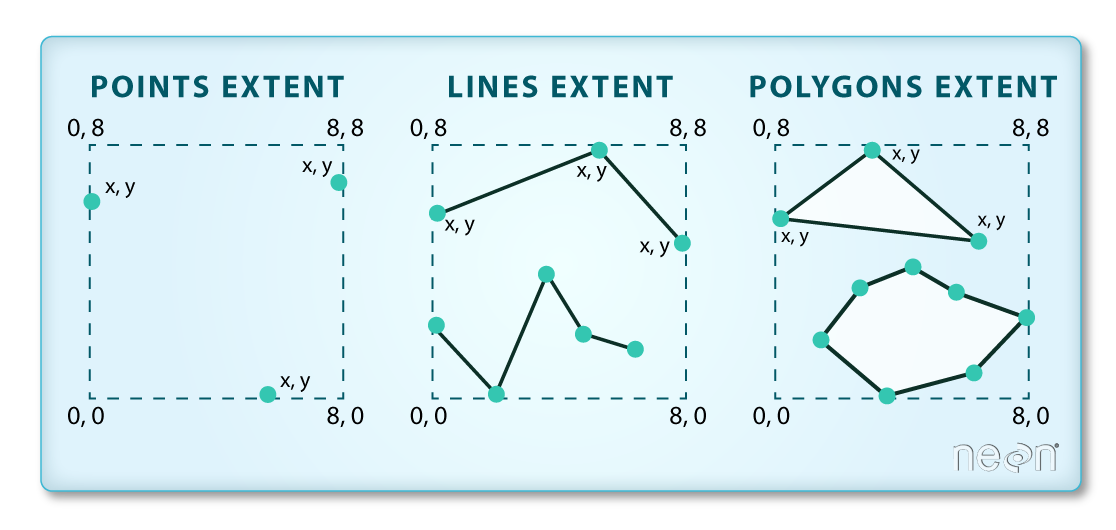
- How can I distinguish between and visualize point, line and polygon vector data?
Objectives
- Know the difference between point, line, and polygon vector elements.
- Load point, line, and polygon vector layers into R.
- Access the attributes of a spatial object in R.
Things You’ll Need To Complete This Episode
See the lesson homepage for detailed information about the software, data, and other prerequisites you will need to work through the examples in this episode.
Starting with this episode, we will be moving from working with
raster data to working with vector data. In this episode, we will open
and plot point, line and polygon vector data loaded from ESRI’s
shapefile format into R. These data refer to the NEON
Harvard Forest field site, which we have been working with in
previous episodes. In later episodes, we will learn how to work with
raster and vector data together and combine them into a single plot.
Import Vector Data
We will use the sf package to work with vector data in
R. We will also use the terra package, which has been
loaded in previous episodes, so we can explore raster and vector spatial
metadata using similar commands. Make sure you have the sf
library loaded.
R
library(sf)
The vector layers that we will import from ESRI’s
shapefile format are:
- A polygon vector layer representing our field site boundary,
- A line vector layer representing roads, and
- A point vector layer representing the location of the Fisher flux tower located at the NEON Harvard Forest field site.
The first vector layer that we will open contains the boundary of our
study area (or our Area Of Interest or AOI, hence the name
aoiBoundary). To import a vector layer from an ESRI
shapefile we use the sf function
st_read(). st_read() requires the file path to
the ESRI shapefile.
Let’s import our AOI:
R
aoi_boundary_HARV <- st_read(
  "data/NEON-DS-Site-Layout-Files/HARV/HarClip_UTMZ18.shp")
OUTPUT
Reading layer `HarClip_UTMZ18' from data source
  `/home/runner/work/r-raster-vector-geospatial/r-raster-vector-geospatial/site/built/data/NEON-DS-Site-Layout-Files/HARV/HarClip_UTMZ18.shp'
  using driver `ESRI Shapefile'
Simple feature collection with 1 feature and 1 field
Geometry type: POLYGON
Dimension:     XY
Bounding box:  xmin: 732128 ymin: 4713209 xmax: 732251.1 ymax: 4713359
Projected CRS: WGS 84 / UTM zone 18N
Vector Layer Metadata & Attributes
When we import the HarClip_UTMZ18 vector layer from an
ESRI shapefile into R (as our
aoi_boundary_HARV object), the st_read()
function automatically stores information about the data. We are
particularly interested in the geospatial metadata, describing the
format, CRS, extent, and other components of the vector data, and the
attributes which describe properties associated with each individual
vector object.
Data Tip
The Explore and Plot by Vector Layer Attributes episode provides more information on both metadata and attributes and using attributes to subset and plot data.
Spatial Metadata
Key metadata for all vector layers includes:
- Object Type: the class of the imported object.
- Coordinate Reference System (CRS): the projection of the data.
- Extent: the spatial extent (i.e. geographic area that the vector layer covers) of the data. Note that the spatial extent for a vector layer represents the combined extent for all individual objects in the vector layer.
We can view metadata of a vector layer using the
st_geometry_type(), st_crs() and
st_bbox() functions. First, let’s view the geometry type
for our AOI vector layer:
R
st_geometry_type(aoi_boundary_HARV)
OUTPUT
[1] POLYGON
18 Levels: GEOMETRY POINT LINESTRING POLYGON MULTIPOINT ... TRIANGLE
Our aoi_boundary_HARV is a polygon spatial object. The
18 levels shown below our output list the possible categories of the
geometry type. Now let’s check what CRS this file data is in:
R
st_crs(aoi_boundary_HARV)
OUTPUT
Coordinate Reference System:
  User input: WGS 84 / UTM zone 18N
  wkt:
PROJCRS["WGS 84 / UTM zone 18N",
    BASEGEOGCRS["WGS 84",
        DATUM["World Geodetic System 1984",
            ELLIPSOID["WGS 84",6378137,298.257223563,
                LENGTHUNIT["metre",1]]],
        PRIMEM["Greenwich",0,
            ANGLEUNIT["degree",0.0174532925199433]],
        ID["EPSG",4326]],
    CONVERSION["UTM zone 18N",
        METHOD["Transverse Mercator",
            ID["EPSG",9807]],
        PARAMETER["Latitude of natural origin",0,
            ANGLEUNIT["Degree",0.0174532925199433],
            ID["EPSG",8801]],
        PARAMETER["Longitude of natural origin",-75,
            ANGLEUNIT["Degree",0.0174532925199433],
            ID["EPSG",8802]],
        PARAMETER["Scale factor at natural origin",0.9996,
            SCALEUNIT["unity",1],
            ID["EPSG",8805]],
        PARAMETER["False easting",500000,
            LENGTHUNIT["metre",1],
            ID["EPSG",8806]],
        PARAMETER["False northing",0,
            LENGTHUNIT["metre",1],
            ID["EPSG",8807]]],
    CS[Cartesian,2],
        AXIS["(E)",east,
            ORDER[1],
            LENGTHUNIT["metre",1]],
        AXIS["(N)",north,
            ORDER[2],
            LENGTHUNIT["metre",1]],
    ID["EPSG",32618]]
Our data in the CRS UTM zone 18N. The CRS is
critical to interpreting the spatial object’s extent values as it
specifies units. To find the extent of our AOI, we can use the
st_bbox() function:
R
st_bbox(aoi_boundary_HARV)
OUTPUT
     xmin      ymin      xmax      ymax
 732128.0 4713208.7  732251.1 4713359.2
The spatial extent of a vector layer or R spatial object represents the geographic “edge” or location that is the furthest north, south east and west. Thus it represents the overall geographic coverage of the spatial object. Image Source: National Ecological Observatory Network (NEON).
Lastly, we can view all of the metadata and attributes for this R spatial object by printing it to the screen:
R
aoi_boundary_HARV
OUTPUT
Simple feature collection with 1 feature and 1 field
Geometry type: POLYGON
Dimension:     XY
Bounding box:  xmin: 732128 ymin: 4713209 xmax: 732251.1 ymax: 4713359
Projected CRS: WGS 84 / UTM zone 18N
  id                       geometry
1  1 POLYGON ((732128 4713359, 7...
Spatial Data Attributes
We introduced the idea of spatial data attributes in an earlier lesson. Now we will explore how to use spatial data attributes stored in our data to plot different features.
Plot a vector layer
Next, let’s visualize the data in our sf object using
the ggplot package. Unlike with raster data, we do not need
to convert vector data to a dataframe before plotting with
ggplot.
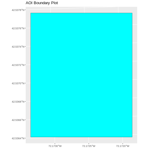
We’re going to customize our boundary plot by setting the size,
color, and fill for our plot. When plotting sf objects with
ggplot2, you need to use the coord_sf()
coordinate system.
R
ggplot() +
  geom_sf(data = aoi_boundary_HARV, size = 3, color = "black", fill = "cyan1") +
  ggtitle("AOI Boundary Plot") +
  coord_sf()
Challenge: Import Line and Point Vector Layers
Using the steps above, import the HARV_roads and HARVtower_UTM18N
vector layers into R. Call the HARV_roads object lines_HARV
and the HARVtower_UTM18N point_HARV.
Answer the following questions:
What type of R spatial object is created when you import each layer?
What is the CRS and extent for each object?
Do the files contain points, lines, or polygons?
How many spatial objects are in each file?
First we import the data:
R
lines_HARV <- st_read("data/NEON-DS-Site-Layout-Files/HARV/HARV_roads.shp")
OUTPUT
Reading layer `HARV_roads' from data source
  `/home/runner/work/r-raster-vector-geospatial/r-raster-vector-geospatial/site/built/data/NEON-DS-Site-Layout-Files/HARV/HARV_roads.shp'
  using driver `ESRI Shapefile'
Simple feature collection with 13 features and 15 fields
Geometry type: MULTILINESTRING
Dimension:     XY
Bounding box:  xmin: 730741.2 ymin: 4711942 xmax: 733295.5 ymax: 4714260
Projected CRS: WGS 84 / UTM zone 18N
R
point_HARV <- st_read("data/NEON-DS-Site-Layout-Files/HARV/HARVtower_UTM18N.shp")
OUTPUT
Reading layer `HARVtower_UTM18N' from data source
  `/home/runner/work/r-raster-vector-geospatial/r-raster-vector-geospatial/site/built/data/NEON-DS-Site-Layout-Files/HARV/HARVtower_UTM18N.shp'
  using driver `ESRI Shapefile'
Simple feature collection with 1 feature and 14 fields
Geometry type: POINT
Dimension:     XY
Bounding box:  xmin: 732183.2 ymin: 4713265 xmax: 732183.2 ymax: 4713265
Projected CRS: WGS 84 / UTM zone 18N
Then we check its class:
R
class(lines_HARV)
OUTPUT
[1] "sf" "data.frame"R
class(point_HARV)
OUTPUT
[1] "sf" "data.frame"We also check the CRS and extent of each object:
R
st_crs(lines_HARV)
OUTPUT
Coordinate Reference System:
  User input: WGS 84 / UTM zone 18N
  wkt:
PROJCRS["WGS 84 / UTM zone 18N",
    BASEGEOGCRS["WGS 84",
        DATUM["World Geodetic System 1984",
            ELLIPSOID["WGS 84",6378137,298.257223563,
                LENGTHUNIT["metre",1]]],
        PRIMEM["Greenwich",0,
            ANGLEUNIT["degree",0.0174532925199433]],
        ID["EPSG",4326]],
    CONVERSION["UTM zone 18N",
        METHOD["Transverse Mercator",
            ID["EPSG",9807]],
        PARAMETER["Latitude of natural origin",0,
            ANGLEUNIT["Degree",0.0174532925199433],
            ID["EPSG",8801]],
        PARAMETER["Longitude of natural origin",-75,
            ANGLEUNIT["Degree",0.0174532925199433],
            ID["EPSG",8802]],
        PARAMETER["Scale factor at natural origin",0.9996,
            SCALEUNIT["unity",1],
            ID["EPSG",8805]],
        PARAMETER["False easting",500000,
            LENGTHUNIT["metre",1],
            ID["EPSG",8806]],
        PARAMETER["False northing",0,
            LENGTHUNIT["metre",1],
            ID["EPSG",8807]]],
    CS[Cartesian,2],
        AXIS["(E)",east,
            ORDER[1],
            LENGTHUNIT["metre",1]],
        AXIS["(N)",north,
            ORDER[2],
            LENGTHUNIT["metre",1]],
    ID["EPSG",32618]]
R
st_bbox(lines_HARV)
OUTPUT
     xmin      ymin      xmax      ymax
 730741.2 4711942.0  733295.5 4714260.0
R
st_crs(point_HARV)
OUTPUT
Coordinate Reference System:
  User input: WGS 84 / UTM zone 18N
  wkt:
PROJCRS["WGS 84 / UTM zone 18N",
    BASEGEOGCRS["WGS 84",
        DATUM["World Geodetic System 1984",
            ELLIPSOID["WGS 84",6378137,298.257223563,
                LENGTHUNIT["metre",1]]],
        PRIMEM["Greenwich",0,
            ANGLEUNIT["degree",0.0174532925199433]],
        ID["EPSG",4326]],
    CONVERSION["UTM zone 18N",
        METHOD["Transverse Mercator",
            ID["EPSG",9807]],
        PARAMETER["Latitude of natural origin",0,
            ANGLEUNIT["Degree",0.0174532925199433],
            ID["EPSG",8801]],
        PARAMETER["Longitude of natural origin",-75,
            ANGLEUNIT["Degree",0.0174532925199433],
            ID["EPSG",8802]],
        PARAMETER["Scale factor at natural origin",0.9996,
            SCALEUNIT["unity",1],
            ID["EPSG",8805]],
        PARAMETER["False easting",500000,
            LENGTHUNIT["metre",1],
            ID["EPSG",8806]],
        PARAMETER["False northing",0,
            LENGTHUNIT["metre",1],
            ID["EPSG",8807]]],
    CS[Cartesian,2],
        AXIS["(E)",east,
            ORDER[1],
            LENGTHUNIT["metre",1]],
        AXIS["(N)",north,
            ORDER[2],
            LENGTHUNIT["metre",1]],
    ID["EPSG",32618]]
R
st_bbox(point_HARV)
OUTPUT
     xmin      ymin      xmax      ymax
 732183.2 4713265.0  732183.2 4713265.0
To see the number of objects in each file, we can look at the output
from when we read these objects into R. lines_HARV contains
13 features (all lines) and point_HARV contains only one
point.
Key Points
- Metadata for vector layers include geometry type, CRS, and extent.
- Load spatial objects into R with the
st_read()function. - Spatial objects can be plotted directly with
ggplotusing thegeom_sf()function. No need to convert to a dataframe.