Summary and Setup
Data Carpentry’s aim is to teach researchers basic concepts, skills, and tools for working with data so that they can get more done in less time, and with less pain.
Interested in teaching these materials? We have an onboarding video available to prepare Instructors to teach these lessons. After watching this video, please contact team@carpentries.org so that we can record your status as an onboarded Instructor. Instructors who have completed onboarding will be given priority status for teaching at centrally-organized Data Carpentry Geospatial workshops.
Getting Started
Data Carpentry’s teaching is hands-on, so participants are encouraged to use their own computers to ensure the proper setup of tools for an efficient workflow. To most effectively use these materials, please make sure to download the data and install everything before working through this lesson.
This workshop assumes no prior experience with the tools covered in
the workshop. However, learners with prior experience working with
geospatial data may be able to skip the Geospatial
Project Organization and Management lesson. Similarly, learners who
have prior experience with the R programming language may
wish to skip the Introduction to
R for Geospatial Data lesson.
To get started, follow the directions in the Setup tab to get access to the required software and data for this workshop.
Data
The data and lessons in this workshop were originally developed through a hackathon funded by the National Ecological Observatory Network (NEON) - an NSF funded observatory in Boulder, Colorado - in collaboration with Data Carpentry, SESYNC and CYVERSE. NEON is collecting data for 30 years to help scientists understand how aquatic and terrestrial ecosystems are changing. The data used in these lessons cover two NEON field sites:
- Harvard Forest (HARV) - Massachusetts, USA - fieldsite description
- San Joaquin Experimental Range (SJER) - California, USA - fieldsite description
There are four data sets included, all of which are available on
Figshare under a CC-BY license. You can download all of the data
used in this workshop by clicking this
download link. Clicking the download link will download all of the
files as a single compressed (.zip) file. To expand this
file, double click the folder icon in your file navigator application
(for Macs, this is the Finder application).
These data files represent the teaching version of the data, with sufficient complexity to teach many aspects of data analysis and management, but with many complexities removed to allow students to focus on the core ideas and skills being taught.
| Dataset | File name | Description |
|---|---|---|
| Site layout shapefiles | NEON-DS-Site-Layout-Files.zip | A set of shapefiles for the NEON’s Harvard Forest field site and US and (some) state boundary layers. |
| Meteorological data | NEON-DS-Met-Time-Series.zip | Precipitation, temperature and other variables collected from a flux tower at the NEON Harvard Forest site |
| Airborne remote sensing data | NEON-DS-Airborne-RemoteSensing.zip | LiDAR data collected by the NEON Airborne Observation Platform (AOP) and processed at NEON including a canopy height model, digital elevation model and digital surface model for NEON’s Harvard Forest and San Joaquin Experimental Range field sites. |
| Landstat 7 NDVI raster data | NEON-DS-Landsat-NDVI.zip | 2011 NDVI data product derived from Landsat 7 and processed by USGS cropped to NEON’s Harvard Forest and San Joaquin Experimental Range field sites |
Workshop Overview
| Lesson | Overview |
|---|---|
| Introduction to Geospatial Concepts | Understand data structures and common storage and transfer formats for spatial data. |
| Introduction to R for Geospatial Data | Import data into R, calculate summary statistics, and create publication-quality graphics. |
| Introduction to Geospatial Raster and Vector Data with R | Open, work with, and plot vector and raster-format spatial data in R. |
Overview
This workshop is designed to be run on your local machine. First, you will need to download the data we use in the workshop. Then, you need to set up your machine to analyze and process geospatial data. We provide instructions below to either install all components manually (option A), or to use a Docker image that provides all the software and dependencies needed (option B).
Data
You can download all of the data used in this workshop by clicking this download link. The file is 218.2 MB.
Clicking the download link will automatically download all of the
files to your default download directory as a single compressed
(.zip) file. To expand this file, double click the folder
icon in your file navigator application (for Macs, this is the Finder
application).
For a full description of the data used in this workshop see the data page.
Option A: Local Installation
Software
| Software | Install | Manual | Available for | Description |
|---|---|---|---|---|
| R | Link | Link | Linux, MacOS | Software environment for statistical and scientific computing |
| RStudio | Link | Linux, MacOS | GUI for R |
We provide quick instructions below for installing the various software needed for this workshop. At points, they assume familiarity with the command line and with installation in general. As there are different operating systems and many different versions of operating systems and environments, these may not work on your computer. If an installation doesn’t work for you, please refer to the installation instructions for that software listed in the table above.
To install the geospatial libraries, install the latest version RTools
The simplest way to install these geospatial libraries is to install
the latest version of Kyng Chaos’s
pre-built package for GDAL Complete. Be aware that several other
libraries are also installed, including the UnixImageIO, SQLite3, and
NumPy.
After downloading the package in the link above, you will need to double-click the cardbord box icon to complete the installation. Depending on your security settings, you may get an error message about “unidentified developers”. You can enable the installation by following these instructions for installing programs from unidentified developers.
Alternatively, participants who are comfortable with the command line can install the geospatial libraries individually using homebrew:
Steps for installing the geospatial libraries will vary based on
which form of Linux you are using. These instructions are adapted from
the sf package’s
README.
For Ubuntu:
BASH
$ sudo add-apt-repository ppa:ubuntugis
$ sudo apt-get update
$ sudo apt-get install libgdal-dev libgeos-dev libproj-dev
For Fedora:
For Arch:
For Debian: The rocker geospatial Dockerfiles may be helpful. Ubuntu Dockerfiles are found here. These may be helpful to get an idea of the commands needed to install the necessary dependencies.
UDUNITS
Linux users will have to install UDUNITS separately. Like the
geospatial libraries discussed above, this is a dependency for the
R package sf. Due to conflicts, it does not
install properly on Linux machines when installed as part of the
sf installation process. It is therefore necessary to
install it using the command line ahead of time.
Steps for installing the geospatial will vary based on which form of
Linux you are using. These instructions are adapted from the sf package’s
README.
For Ubuntu:
For Fedora:
For Arch:
For Debian:
R
Participants who do not already have R installed should
download and install it.
To install R, Windows users should select “Download R
for Windows” from RStudio and CRAN’s cloud download page, which will
automatically detect a CRAN mirror for you to use. Select the
base subdirectory after choosing the Windows download page.
A .exe executable file containing the necessary components
of base R can be downloaded by clicking on “Download R 3.x.x for
Windows”.
To install R, macOS users should select “Download R for
(Mac) OS X” from RStudio and CRAN’s cloud download page, which will
automatically detect a CRAN mirror for you to use. A .pkg
file containing the necessary components of base R can be downloaded by
clicking on the first available link (this will be the most recent),
which will read R-3.x.x.pkg.
To install R, Linux users should select “Download R for
Linux” from RStudio and CRAN’s cloud download page, which will
automatically detect a CRAN mirror for you to use. Instructions for a
number of different Linux operating systems are available.
RStudio
RStudio is a GUI for using R that is available for
Windows, macOS, and various Linux operating systems. It can be
downloaded here. You
will need the free Desktop version for your computer.
In order to address issues with ggplot2, learners and
instructors should run a recent version of RStudio (v1.2 or
greater).
R Packages
The following R packages are used in the various
geospatial lessons.
To install these packages in RStudio, do the following:
1. Open RStudio by double-clicking the RStudio application icon. You
should see something like this:
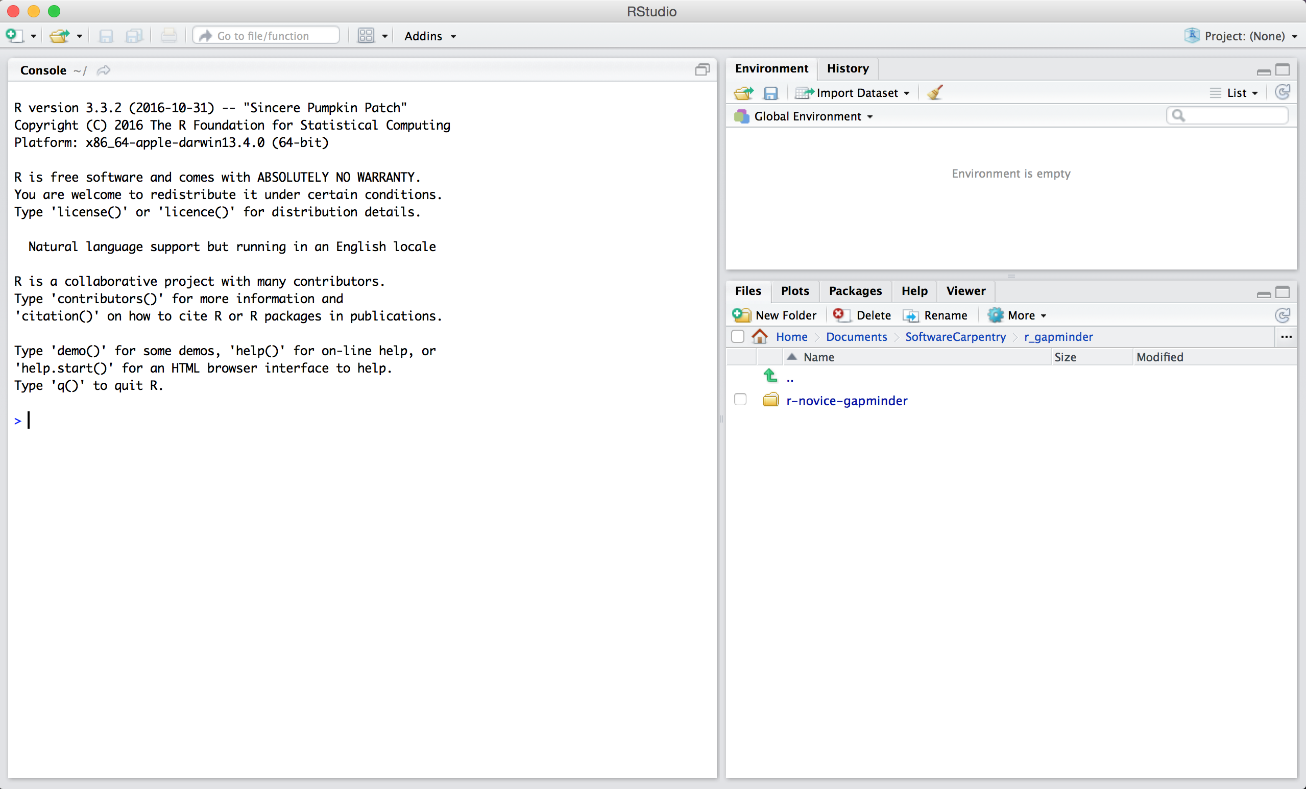
2. Type the following into the console and hit enter.
R
install.packages(c("dplyr", "ggplot2", "raster", "rasterVis", "RColorBrewer", "remotes", "reshape", "scales", "sf", "terra", "tidyr"))
You should see a status message starting with:
OUTPUT
trying URL 'https://cran.rstudio.com/bin/macosx/el-capitan/contrib/3.5/dplyr_0.7.6.tgz'
Content type 'application/x-gzip' length 5686536 bytes (5.4 MB)
==================================================
downloaded 5.4 MB

trying URL 'https://cran.rstudio.com/bin/macosx/el-capitan/contrib/3.5/ggplot2_3.0.0.tgz'
Content type 'application/x-gzip' length 3577658 bytes (3.4 MB)
==================================================
downloaded 3.4 MB
When the installation is complete, you will see a status message like:
OUTPUT
The downloaded binary packages are in
/var/folders/7g/r8_n81y534z0vy5hxc6dx1t00000gn/T//RtmpJECKXM/downloaded_packages
You are now ready for the workshop!
Option B: Docker
Docker provides developers with
a means for creating interactive containers
that contain pre-installed software. A selection of pre-installed
software in Docker is called an image. An image
can be downloaded and used to create a local container, allowing
end-users to get software up and running quickly. This is particularly
useful when a local installation of the software could be complex and
time consuming. For R users, a Docker image can be used to
create a virtual installation of R and RStudio that can be
run through your web browser.
This option involves downloading an Docker image that contains an
installation of R, RStudio Server, all of the necessary
dependencies listed above, and almost all of the R packages
used in the geospatial lessons. You will need to install the appropriate
version of Docker’s Community Edition software and then download and use
the rocker/geospatial Docker image to create a container
that will allow you to use R, RStudio, and all the required
GIS tools without installing any of them locally.
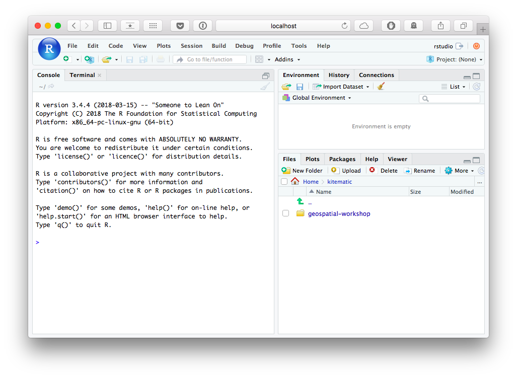
Once up and running - you’ll have full access to RStudio right from your browser:
Please be aware that the R package
rasterVis is not included in the
rocker/geospatial Docker image. If your instructor teaches
with this package then you will need to install this R
package yourself. All other R packages will already be
installed for you.
To get started with Docker, download the Docker Community Edition from Docker’s store. Community editions are available for Windows, macOS, and Linux operating systems including Debian, Fedora, and Ubuntu.
The download pages for each of these operating systems contain notes about some necessary system requirements and other pre-requisites. Once you download the installer and follow the on-screen prompts.
Additional installation notes are available in Docker’s documentation for each of these operating systems: Windows, macOS, Debian, Fedora, and Ubuntu.
Download and Set-up
Once Docker is installed and up and running, you will need to open
your computer’s command line terminal. We’ll use the terminal to
download rocker/geospatial,
a pre-made Docker image that contains an installation of R,
RStudio Server, all of the necessary dependencies, and all but one of
the R packages needed for this workshop.
You need to have already installed Docker Community Edition (see
instructions above) before proceeding. Once you have Docker downloaded
and installed, make sure Docker is running and then enter the following
command into the terminal to download the rocker/geospatial
image:
Once the pull command is executed, the image needs to be run to
become accessible as a container. In the following example, the image is
named rocker/geospatial and the container is named
gis. The image contains
the software you’ve downloaded, and the container is
the run-time instance of that image. New Docker users should need only
one named container per image.
When docker run is used, you can specify a folder on
your computer to become accessible inside your RStudio Server instance.
The following docker run command exposes Jane’s
GitHub directory to RStudio Server. Enter the file path
where your workshop resources and data are stored:
BASH
$ docker run -d -P --name gis -v /Users/jane/GitHub:/home/rstudio/GitHub -e PASSWORD=mypass rocker/geospatialWhen she opens her RStudio instance below, she will see a
GitHub folder in her file tab in the lower righthand corner
of the screen. Windows and Linux users will have to adapt the file path
above to follow the standards of their operating systems. More details
are available on rocker’s
Wiki.
The last step before launching your container in a browser is to identify the port that your Docker container is running in:
An output, for example, of 8787/tcp -> 0.0.0.0:32768
would indicate that you should point your browser to
http://localhost:32768/. If prompted, enter
rstudio for the username and the password provided in the
docker run command above (mypass in the
example above).
Stopping a Container
When you are done with a Docker session, make sure all of your files
are saved locally on your computer before closing your browser
and Docker. Once you have ensured all of your files are
available (they should be saved at the file path designated in
docker run above), you can stop your Docker container in
the terminal:
Re-starting a Container
Once a container has been named and created, you cannot create a
container with the same name again using docker run.
Instead, you can restart it:
If you cannot remember the name of the container you created, you can use the following command to print a list of all named containers:
If you are returning to a session after stopping Docker itself, make sure Docker is running again before re-starting your container!
Download and Install Kitematic
Kitematic is the GUI, currently in beta, that Docker has built for accessing images and containers on Windows, macOS, and Ubuntu. You can download the appropriate installer files from Kitematic’s GitHub release page. You need to have already installed Docker Community Edition (see instructions above) before installing Kitematic!
Opening a Container with Kitematic
Once you have installed Kitematic, make sure the Docker application
is running and then open Kitematic. You should not need to create a
login to use Kitematic. If prompted for login credentials, there is an
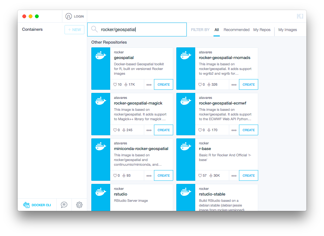
option to skip that step. Use the search bar in the main window to find
rocker/geospatial (pictured below) and click
Create under that Docker repository.
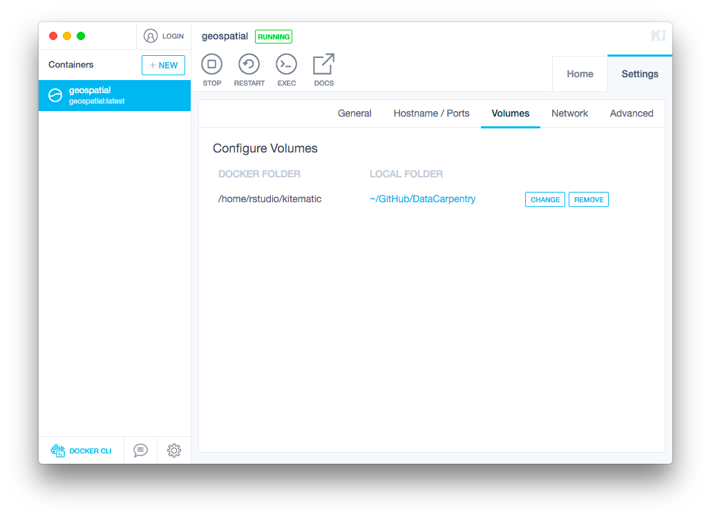
After downloading and installing the image, your container should
start automatically. Before opening your browser, connect your Docker
image to a local folder where you have your workshop resources stored by
clicking on the Settings tab and then choosing
Volumes. Click Change and then select the
directory you would like to connect to.
When you open RStudio instance below, you will see the contents of
the connected folder inside the kitematic directory in the
file tab located in the lower righthand corner of the screen.
When you are ready, copy the Access URL from the
Home tab:
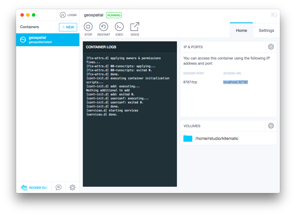
Paste that url into your browser and, if prompted, enter
rstudio for both the username and the password.
Stopping and Restarting a Container
When you are done with a Docker session, make sure all of your files
are saved locally on your computer before closing your browser
and Docker. Once you have ensured all of your files are
available (they should be saved at the file path designated in
docker run above), you can stop your Docker container by
clicking on the Stop icon in Kitematic’s toolbar.
You can restart your container later by clicking the
Restart button.
To obtain a list of all of your current Docker containers:
To list all of the currently downloaded Docker images:
These images can take up system resources, and if you’d like to
remove them, you can use the docker prune command. To
remove any Docker resources not affiliated with a container listed under
docker ps -a:
To remove all Docker resources, including currently named containers: