Plot Multiple Vector Layers
Last updated on 2024-10-15 | Edit this page
Overview
Questions
- How can I create map compositions with custom legends using ggplot?
- How can I plot raster and vector data together?
Objectives
- Plot multiple vector layers in the same plot.
- Apply custom symbols to spatial objects in a plot.
- Create a multi-layered plot with raster and vector data.
Things You’ll Need To Complete This Episode
See the lesson homepage for detailed information about the software, data, and other prerequisites you will need to work through the examples in this episode.
This episode builds upon the previous episode to work with vector layers in R and explore how to plot multiple vector layers. It also covers how to plot raster and vector data together on the same plot.
Load the Data
To work with vector data in R, we can use the sf
library. The terra package also allows us to explore
metadata using similar commands for both raster and vector files. Make
sure that you have these packages loaded.
We will continue to work with the three ESRI shapefile
that we loaded in the Open and
Plot Vector Layers in R episode.
Plotting Multiple Vector Layers
In the previous episode, we learned how to plot information from a single vector layer and do some plot customization including adding a custom legend. However, what if we want to create a more complex plot with many vector layers and unique symbols that need to be represented clearly in a legend?
Now, let’s create a plot that combines our tower location
(point_HARV), site boundary
(aoi_boundary_HARV) and roads (lines_HARV)
spatial objects. We will need to build a custom legend as well.
To begin, we will create a plot with the site boundary as the first
layer. Then layer the tower location and road data on top using
+.
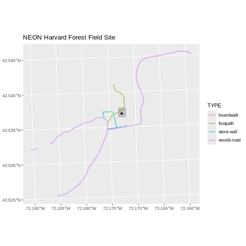
R
ggplot() +
  geom_sf(data = aoi_boundary_HARV, fill = "grey", color = "grey") +
  geom_sf(data = lines_HARV, aes(color = TYPE), size = 1) +
  geom_sf(data = point_HARV) +
  ggtitle("NEON Harvard Forest Field Site") +
  coord_sf()
Next, let’s build a custom legend using the symbology (the colors and
symbols) that we used to create the plot above. For example, it might be
good if the lines were symbolized as lines. In the previous episode, you
may have noticed that the default legend behavior for
geom_sf is to draw a ‘patch’ for each legend entry. If you
want the legend to draw lines or points, you need to add an instruction
to the geom_sf call - in this case,
show.legend = 'line'.
R
ggplot() +
  geom_sf(data = aoi_boundary_HARV, fill = "grey", color = "grey") +
  geom_sf(data = lines_HARV, aes(color = TYPE),
          show.legend = "line", size = 1) +
  geom_sf(data = point_HARV, aes(fill = Sub_Type), color = "black") +
  scale_color_manual(values = road_colors) +
  scale_fill_manual(values = "black") +
  ggtitle("NEON Harvard Forest Field Site") +
  coord_sf()
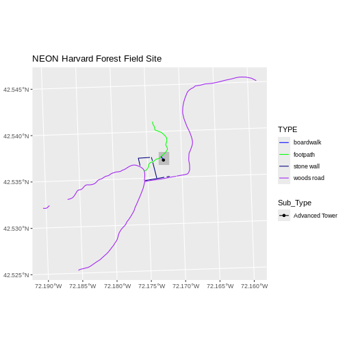
Now lets adjust the legend titles by passing a name to
the respective color and fill palettes.
R
ggplot() +
  geom_sf(data = aoi_boundary_HARV, fill = "grey", color = "grey") +
  geom_sf(data = point_HARV, aes(fill = Sub_Type)) +
  geom_sf(data = lines_HARV, aes(color = TYPE), show.legend = "line",
          size = 1) +
  scale_color_manual(values = road_colors, name = "Line Type") +
  scale_fill_manual(values = "black", name = "Tower Location") +
  ggtitle("NEON Harvard Forest Field Site") +
  coord_sf()

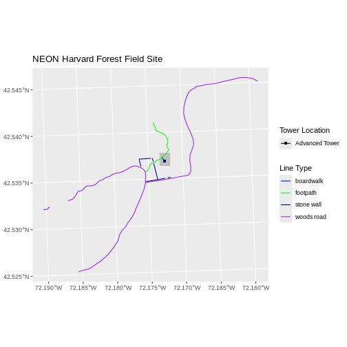
Finally, it might be better if the points were symbolized as a
symbol. We can customize this using shape parameters in our
call to geom_sf: 16 is a point symbol, 15 is a box.
Data Tip
To view a short list of shape symbols, type
?pch into the R console.
R
ggplot() +
  geom_sf(data = aoi_boundary_HARV, fill = "grey", color = "grey") +
  geom_sf(data = point_HARV, aes(fill = Sub_Type), shape = 15) +
  geom_sf(data = lines_HARV, aes(color = TYPE),
          show.legend = "line", size = 1) +
  scale_color_manual(values = road_colors, name = "Line Type") +
  scale_fill_manual(values = "black", name = "Tower Location") +
  ggtitle("NEON Harvard Forest Field Site") +
  coord_sf()
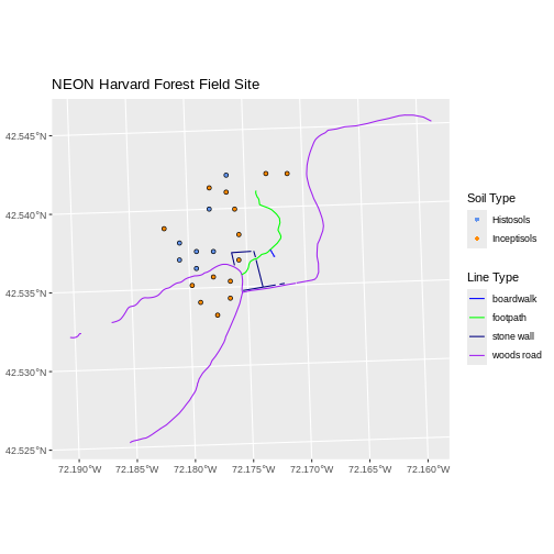
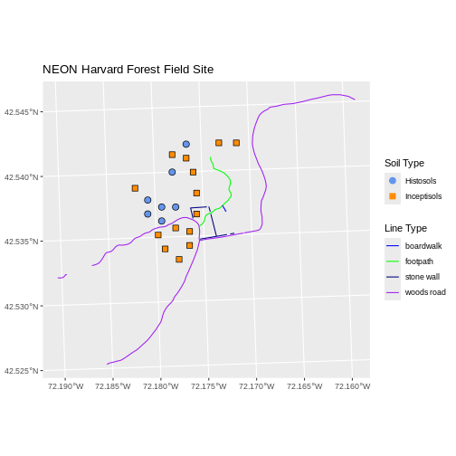
Challenge: Plot Polygon by Attribute
Using the
NEON-DS-Site-Layout-Files/HARV/PlotLocations_HARV.shpESRIshapefile, create a map of study plot locations, with each point colored by the soil type (soilTypeOr). How many different soil types are there at this particular field site? Overlay this layer on top of thelines_HARVlayer (the roads). Create a custom legend that applies line symbols to lines and point symbols to the points.Modify the plot above. Tell R to plot each point, using a different symbol of
shapevalue.
First we need to read in the data and see how many unique soils are
represented in the soilTypeOr attribute.
R
plot_locations <-
  st_read("data/NEON-DS-Site-Layout-Files/HARV/PlotLocations_HARV.shp")
OUTPUT
Reading layer `PlotLocations_HARV' from data source
  `/home/runner/work/r-raster-vector-geospatial/r-raster-vector-geospatial/site/built/data/NEON-DS-Site-Layout-Files/HARV/PlotLocations_HARV.shp'
  using driver `ESRI Shapefile'
Simple feature collection with 21 features and 25 fields
Geometry type: POINT
Dimension:     XY
Bounding box:  xmin: 731405.3 ymin: 4712845 xmax: 732275.3 ymax: 4713846
Projected CRS: WGS 84 / UTM zone 18N
R
plot_locations$soilTypeOr <- as.factor(plot_locations$soilTypeOr)
levels(plot_locations$soilTypeOr)
OUTPUT
[1] "Histosols" "Inceptisols"Next we can create a new color palette with one color for each soil type.
R
blue_orange <- c("cornflowerblue", "darkorange")
Finally, we will create our plot.
R
ggplot() +
  geom_sf(data = lines_HARV, aes(color = TYPE), show.legend = "line") +
  geom_sf(data = plot_locations, aes(fill = soilTypeOr),
          shape = 21, show.legend = 'point') +
  scale_color_manual(name = "Line Type", values = road_colors,
     guide = guide_legend(override.aes = list(linetype = "solid",
                                              shape = NA))) +
  scale_fill_manual(name = "Soil Type", values = blue_orange,
     guide = guide_legend(override.aes = list(linetype = "blank", shape = 21,
                                              colour = NA))) +
  ggtitle("NEON Harvard Forest Field Site") +
  coord_sf()
If we want each soil to be shown with a different symbol, we can give
multiple values to the scale_shape_manual() argument.
R
ggplot() +
  geom_sf(data = lines_HARV, aes(color = TYPE), show.legend = "line", size = 1) +
  geom_sf(data = plot_locations, aes(fill = soilTypeOr, shape = soilTypeOr),
          show.legend = 'point', size = 3) +
  scale_shape_manual(name = "Soil Type", values = c(21, 22)) +
  scale_color_manual(name = "Line Type", values = road_colors,
     guide = guide_legend(override.aes = list(linetype = "solid", shape = NA))) +
  scale_fill_manual(name = "Soil Type", values = blue_orange,
     guide = guide_legend(override.aes = list(linetype = "blank", shape = c(21, 22),
     color = blue_orange))) +
  ggtitle("NEON Harvard Forest Field Site") +
  coord_sf()
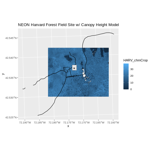
Challenge: Plot Raster & Vector Data Together
You can plot vector data layered on top of raster data using the
+ to add a layer in ggplot. Create a plot that
uses the NEON AOI Canopy Height Model
data/NEON-DS-Airborne-Remote-Sensing/HARV/CHM/HARV_chmCrop.tif
as a base layer. On top of the CHM, please add:
- The study site AOI.
- Roads.
- The tower location.
Be sure to give your plot a meaningful title.
R
ggplot() +
  geom_raster(data = CHM_HARV_df, aes(x = x, y = y, fill = HARV_chmCrop)) +
  geom_sf(data = lines_HARV, color = "black") +
  geom_sf(data = aoi_boundary_HARV, color = "grey20", size = 1) +
  geom_sf(data = point_HARV, pch = 8) +
  ggtitle("NEON Harvard Forest Field Site w/ Canopy Height Model") +
  coord_sf()
Key Points
- Use the
+operator to add multiple layers to a ggplot. - Multi-layered plots can combine raster and vector datasets.
- Use the
show.legendargument to set legend symbol types. - Use the
scale_fill_manual()function to set legend colors.