Derive Values from Raster Time Series
Last updated on 2024-10-15 | Edit this page
Overview
Questions
- How can I calculate, extract, and export summarized raster pixel data?
Objectives
- Extract summary pixel values from a raster.
- Save summary values to a .csv file.
- Plot summary pixel values using
ggplot(). - Compare NDVI values between two different sites.
Things You’ll Need To Complete This Episode
See the lesson homepage for detailed information about the software, data, and other prerequisites you will need to work through the examples in this episode.
In this episode, we will extract NDVI values from a raster time
series dataset and plot them using the ggplot2 package.
Extract Summary Statistics From Raster Data
We often want to extract summary values from raster data. For example, we might want to understand overall greeness across a field site or at each plot within a field site. These values can then be compared between different field sites and combined with other related metrics to support modeling and further analysis.
Calculate Average NDVI
Our goal in this episode is to create a dataframe that contains a single, mean NDVI value for each raster in our time series. This value represents the mean NDVI value for this area on a given day.
We can calculate the mean for each raster using the
global() function. The global() function
produces a named numeric vector, where each value is associated with the
name of raster stack it was derived from.
R
avg_NDVI_HARV <- global(NDVI_HARV_stack, mean)
avg_NDVI_HARV
OUTPUT
                        mean
X005_HARV_ndvi_crop 0.365150
X037_HARV_ndvi_crop 0.242645
X085_HARV_ndvi_crop 0.251390
X133_HARV_ndvi_crop 0.599300
X181_HARV_ndvi_crop 0.878725
X197_HARV_ndvi_crop 0.893250
X213_HARV_ndvi_crop 0.878395
X229_HARV_ndvi_crop 0.881505
X245_HARV_ndvi_crop 0.850120
X261_HARV_ndvi_crop 0.796360
X277_HARV_ndvi_crop 0.033050
X293_HARV_ndvi_crop 0.056895
X309_HARV_ndvi_crop 0.541130
The output is a data frame (othewise, we could use
as.data.frame()). It’s a good idea to view the first few
rows of our data frame with head() to make sure the
structure is what we expect.
R
head(avg_NDVI_HARV)
OUTPUT
                        mean
X005_HARV_ndvi_crop 0.365150
X037_HARV_ndvi_crop 0.242645
X085_HARV_ndvi_crop 0.251390
X133_HARV_ndvi_crop 0.599300
X181_HARV_ndvi_crop 0.878725
X197_HARV_ndvi_crop 0.893250
We now have a data frame with row names that are based on the original file name and a mean NDVI value for each file. Next, let’s clean up the column names in our data frame to make it easier for colleagues to work with our code.
Let’s change the NDVI column name to meanNDVI.
R
names(avg_NDVI_HARV) <- "meanNDVI"
head(avg_NDVI_HARV)
OUTPUT
                    meanNDVI
X005_HARV_ndvi_crop 0.365150
X037_HARV_ndvi_crop 0.242645
X085_HARV_ndvi_crop 0.251390
X133_HARV_ndvi_crop 0.599300
X181_HARV_ndvi_crop 0.878725
X197_HARV_ndvi_crop 0.893250
The new column name doesn’t reminds us what site our data are from. While we are only working with one site now, we might want to compare several sites worth of data in the future. Let’s add a column to our dataframe called “site”.
R
avg_NDVI_HARV$site <- "HARV"
We can populate this column with the site name - HARV. Let’s also create a year column and populate it with 2011 - the year our data were collected.
R
avg_NDVI_HARV$year <- "2011"
head(avg_NDVI_HARV)
OUTPUT
                    meanNDVI site year
X005_HARV_ndvi_crop 0.365150 HARV 2011
X037_HARV_ndvi_crop 0.242645 HARV 2011
X085_HARV_ndvi_crop 0.251390 HARV 2011
X133_HARV_ndvi_crop 0.599300 HARV 2011
X181_HARV_ndvi_crop 0.878725 HARV 2011
X197_HARV_ndvi_crop 0.893250 HARV 2011
We now have a dataframe that contains a row for each raster file
processed, and columns for meanNDVI, site, and
year.
Extract Julian Day from row names
We’d like to produce a plot where Julian days (the numeric day of the year, 0 - 365/366) are on the x-axis and NDVI is on the y-axis. To create this plot, we’ll need a column that contains the Julian day value.
One way to create a Julian day column is to use gsub()
on the file name in each row. We can replace both the X and
the _HARV_NDVI_crop to extract the Julian Day value, just
like we did in the previous
episode.
This time we will use one additional trick to do both of these steps
at the same time. The vertical bar character ( | ) is
equivalent to the word “or”. Using this character in our search pattern
allows us to search for more than one pattern in our text strings.
R
julianDays <- gsub("X|_HARV_ndvi_crop", "", row.names(avg_NDVI_HARV))
julianDays
OUTPUT
 [1] "005" "037" "085" "133" "181" "197" "213" "229" "245" "261" "277" "293"
[13] "309"
Now that we’ve extracted the Julian days from our row names, we can add that data to the data frame as a column called “julianDay”.
R
avg_NDVI_HARV$julianDay <- julianDays
Let’s check the class of this new column:
R
class(avg_NDVI_HARV$julianDay)
OUTPUT
[1] "character"Convert Julian Day to Date Class
Currently, the values in the Julian day column are stored as class
character. Storing this data as a date object is better -
for plotting, data subsetting and working with our data. Let’s convert.
We worked with data conversions in an
earlier episode. For an introduction to date-time classes, see the
NEON Data Skills tutorial Convert
Date & Time Data from Character Class to Date-Time Class (POSIX) in
R.
To convert a Julian day number to a date class, we need to set the origin, which is the day that our Julian days start counting from. Our data is from 2011 and we know that the USGS Landsat Team created Julian day values for this year. Therefore, the first day or “origin” for our Julian day count is 01 January 2011.
R
origin <- as.Date("2011-01-01")
Next we convert the julianDay column from character to
integer.
R
avg_NDVI_HARV$julianDay <- as.integer(avg_NDVI_HARV$julianDay)
Once we set the Julian day origin, we can add the Julian day value (as an integer) to the origin date.
Note that when we convert our integer class julianDay
values to dates, we subtracted 1. This is because the origin day is 01
January 2011, so the extracted day is 01. The Julian Day (or year day)
for this is also 01. When we convert from the integer 05
julianDay value (indicating 5th of January), we cannot
simply add origin + julianDay because
01 + 05 = 06 or 06 January 2011. To correct, this error we
then subtract 1 to get the correct day, January 05 2011.
R
avg_NDVI_HARV$Date<- origin + (avg_NDVI_HARV$julianDay - 1)
head(avg_NDVI_HARV$Date)
OUTPUT
[1] "2011-01-05" "2011-02-06" "2011-03-26" "2011-05-13" "2011-06-30"
[6] "2011-07-16"
Since the origin date was originally set as a Date class object, the
new Date column is also stored as class
Date.
R
class(avg_NDVI_HARV$Date)
OUTPUT
[1] "Date"Challenge: NDVI for the San Joaquin Experimental Range
We often want to compare two different sites. The National Ecological Observatory Network (NEON) also has a field site in Southern California at the San Joaquin Experimental Range (SJER).
For this challenge, create a dataframe containing the mean NDVI
values and the Julian days the data was collected (in date format) for
the NEON San Joaquin Experimental Range field site. NDVI data for SJER
are located in the NEON-DS-Landsat-NDVI/SJER/2011/NDVI
directory.
First we will read in the NDVI data for the SJER field site.
R
NDVI_path_SJER <- "data/NEON-DS-Landsat-NDVI/SJER/2011/NDVI"

all_NDVI_SJER <- list.files(NDVI_path_SJER,
                            full.names = TRUE,
                            pattern = ".tif$")

NDVI_stack_SJER <- rast(all_NDVI_SJER)
names(NDVI_stack_SJER) <- paste0("X", names(NDVI_stack_SJER))

NDVI_stack_SJER <- NDVI_stack_SJER/10000
Then we can calculate the mean values for each day and put that in a dataframe.
R
avg_NDVI_SJER <- as.data.frame(global(NDVI_stack_SJER, mean))
Next we rename the NDVI column, and add site and year columns to our data.
R
names(avg_NDVI_SJER) <- "meanNDVI"
avg_NDVI_SJER$site <- "SJER"
avg_NDVI_SJER$year <- "2011"
Now we will create our Julian day column
R
julianDays_SJER <- gsub("X|_SJER_ndvi_crop", "", row.names(avg_NDVI_SJER))
origin <- as.Date("2011-01-01")
avg_NDVI_SJER$julianDay <- as.integer(julianDays_SJER)

avg_NDVI_SJER$Date <- origin + (avg_NDVI_SJER$julianDay - 1)

head(avg_NDVI_SJER)
OUTPUT
                    meanNDVI site year julianDay       Date
X014_SJER_ndvi_crop 0.048216 SJER 2011        14 2011-01-14
X046_SJER_ndvi_crop 0.529780 SJER 2011        46 2011-02-15
X062_SJER_ndvi_crop 0.554368 SJER 2011        62 2011-03-03
X094_SJER_ndvi_crop 0.601096 SJER 2011        94 2011-04-04
X110_SJER_ndvi_crop 0.555836 SJER 2011       110 2011-04-20
X126_SJER_ndvi_crop 0.538336 SJER 2011       126 2011-05-06
Plot NDVI Using ggplot
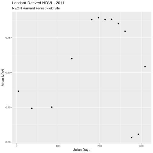
We now have a clean dataframe with properly scaled NDVI and Julian days. Let’s plot our data.
R
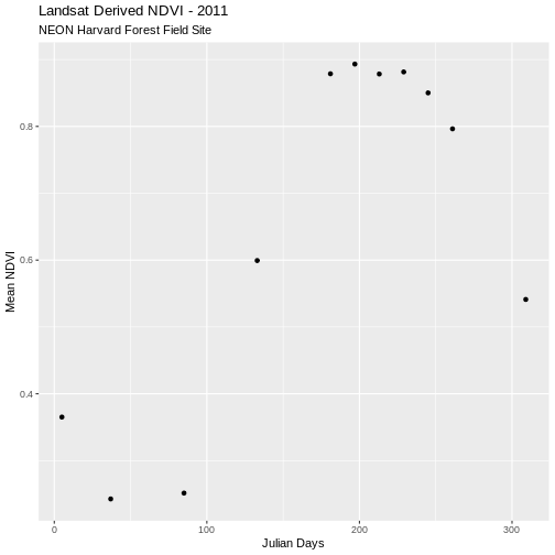
ggplot(avg_NDVI_HARV, aes(julianDay, meanNDVI)) +
  geom_point() +
  ggtitle("Landsat Derived NDVI - 2011",
          subtitle = "NEON Harvard Forest Field Site") +
  xlab("Julian Days") + ylab("Mean NDVI")
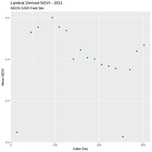
Challenge: Plot San Joaquin Experimental Range Data
Create a complementary plot for the SJER data. Plot the data points in a different color.
R
ggplot(avg_NDVI_SJER, aes(julianDay, meanNDVI)) +
  geom_point(colour = "SpringGreen4") +
  ggtitle("Landsat Derived NDVI - 2011", subtitle = "NEON SJER Field Site") +
  xlab("Julian Day") + ylab("Mean NDVI")
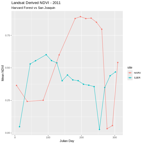
Compare NDVI from Two Different Sites in One Plot
Comparison of plots is often easiest when both plots are side by side. Or, even better, if both sets of data are plotted in the same plot. We can do this by merging the two data sets together. The date frames must have the same number of columns and exact same column names to be merged.
R
NDVI_HARV_SJER <- rbind(avg_NDVI_HARV, avg_NDVI_SJER)
Now we can plot both datasets on the same plot.
R
ggplot(NDVI_HARV_SJER, aes(x = julianDay, y = meanNDVI, colour = site)) +
  geom_point(aes(group = site)) +
  geom_line(aes(group = site)) +
  ggtitle("Landsat Derived NDVI - 2011",
          subtitle = "Harvard Forest vs San Joaquin") +
  xlab("Julian Day") + ylab("Mean NDVI")
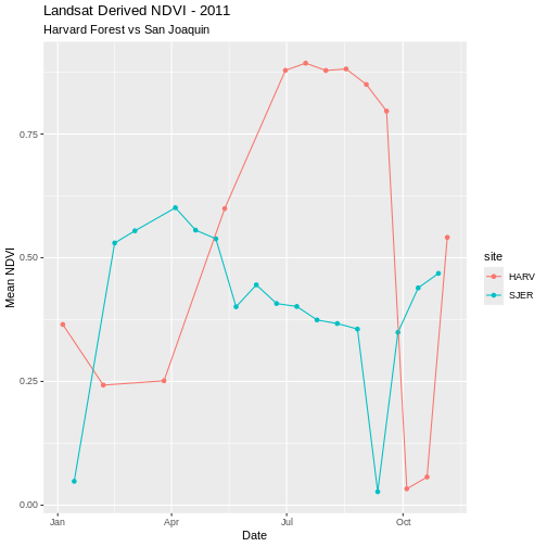
Challenge: Plot NDVI with date
Plot the SJER and HARV data in one plot but use date, rather than Julian day, on the x-axis.
R
ggplot(NDVI_HARV_SJER, aes(x = Date, y = meanNDVI, colour = site)) +
  geom_point(aes(group = site)) +
  geom_line(aes(group = site)) +
  ggtitle("Landsat Derived NDVI - 2011",
          subtitle = "Harvard Forest vs San Joaquin") +
  xlab("Date") + ylab("Mean NDVI")
Remove Outlier Data
As we look at these plots we see variation in greenness across the year. However, the pattern is interrupted by a few points where NDVI quickly drops towards 0 during a time period when we might expect the vegetation to have a higher greenness value. Is the vegetation truly senescent or gone or are these outlier values that should be removed from the data?
We’ve seen in an earlier episode that data points with very low NDVI values can be associated with images that are filled with clouds. Thus, we can attribute the low NDVI values to high levels of cloud cover. Is the same thing happening at SJER?
Without significant additional processing, we will not be able to retrieve a strong reflection from vegetation, from a remotely sensed image that is predominantly cloud covered. Thus, these points are likely bad data points. Let’s remove them.
First, we will identify the good data points that should be retained. One way to do this is by identifying a threshold value. All values below that threshold will be removed from our analysis. We will use 0.1 as an example for this episode. We can then use the subset function to remove outlier datapoints (below our identified threshold).
Data Tip
Thresholding, or removing outlier data, can be tricky business. In this case, we can be confident that some of our NDVI values are not valid due to cloud cover. However, a threshold value may not always be sufficient given that 0.1 could be a valid NDVI value in some areas. This is where decision-making should be fueled by practical scientific knowledge of the data and the desired outcomes!
R
avg_NDVI_HARV_clean <- subset(avg_NDVI_HARV, meanNDVI > 0.1)
avg_NDVI_HARV_clean$meanNDVI < 0.1
OUTPUT
[1] FALSE FALSE FALSE FALSE FALSE FALSE FALSE FALSE FALSE FALSE FALSENow we can create another plot without the suspect data.
R
ggplot(avg_NDVI_HARV_clean, aes(x = julianDay, y = meanNDVI)) +
  geom_point() +
  ggtitle("Landsat Derived NDVI - 2011",
          subtitle = "NEON Harvard Forest Field Site") +
  xlab("Julian Days") + ylab("Mean NDVI")
Now our outlier data points are removed and the pattern of “green-up” and “brown-down” makes more sense.
Write NDVI data to a .csv File
We can write our final NDVI dataframe out to a text format, to quickly share with a colleague or to reuse for analysis or visualization purposes. We will export in Comma Seperated Value (.csv) file format because it is usable in many different tools and across platforms (MAC, PC, etc).
We will use write.csv() to write a specified dataframe
to a .csv file. Unless you designate a different directory,
the output file will be saved in your working directory.
Before saving our file, let’s view the format to make sure it is what we want as an output format.
R
head(avg_NDVI_HARV_clean)
OUTPUT
                    meanNDVI site year julianDay       Date
X005_HARV_ndvi_crop 0.365150 HARV 2011         5 2011-01-05
X037_HARV_ndvi_crop 0.242645 HARV 2011        37 2011-02-06
X085_HARV_ndvi_crop 0.251390 HARV 2011        85 2011-03-26
X133_HARV_ndvi_crop 0.599300 HARV 2011       133 2011-05-13
X181_HARV_ndvi_crop 0.878725 HARV 2011       181 2011-06-30
X197_HARV_ndvi_crop 0.893250 HARV 2011       197 2011-07-16
It looks like we have a series of row.names that we do
not need because we have this information stored in individual columns
in our data frame. Let’s remove the row names.
R
row.names(avg_NDVI_HARV_clean) <- NULL
head(avg_NDVI_HARV_clean)
OUTPUT
  meanNDVI site year julianDay       Date
1 0.365150 HARV 2011         5 2011-01-05
2 0.242645 HARV 2011        37 2011-02-06
3 0.251390 HARV 2011        85 2011-03-26
4 0.599300 HARV 2011       133 2011-05-13
5 0.878725 HARV 2011       181 2011-06-30
6 0.893250 HARV 2011       197 2011-07-16
R
write.csv(avg_NDVI_HARV_clean, file="meanNDVI_HARV_2011.csv")
Challenge: Write to .csv
- Create a NDVI .csv file for the NEON SJER field site that is comparable with the one we just created for the Harvard Forest. Be sure to inspect for questionable values before writing any data to a .csv file.
- Create a NDVI .csv file that includes data from both field sites.
R
avg_NDVI_SJER_clean <- subset(avg_NDVI_SJER, meanNDVI > 0.1)
row.names(avg_NDVI_SJER_clean) <- NULL
head(avg_NDVI_SJER_clean)
OUTPUT
  meanNDVI site year julianDay       Date
1 0.529780 SJER 2011        46 2011-02-15
2 0.554368 SJER 2011        62 2011-03-03
3 0.601096 SJER 2011        94 2011-04-04
4 0.555836 SJER 2011       110 2011-04-20
5 0.538336 SJER 2011       126 2011-05-06
6 0.400868 SJER 2011       142 2011-05-22
R
write.csv(avg_NDVI_SJER_clean, file = "meanNDVI_SJER_2011.csv")
Key Points
- Use the
global()function to calculate summary statistics for cells in a raster object. - The pipe (
|) operator meansor. - Use the
rbind()function to combine data frames that have the same column names.