Reproject Raster Data
Last updated on 2024-10-15 | Edit this page
Overview
Questions
- How do I work with raster data sets that are in different projections?
Objectives
- Reproject a raster in R.
Things You’ll Need To Complete This Episode
See the lesson homepage for detailed information about the software, data, and other prerequisites you will need to work through the examples in this episode.
Sometimes we encounter raster datasets that do not “line up” when
plotted or analyzed. Rasters that don’t line up are most often in
different Coordinate Reference Systems (CRS). This episode explains how
to deal with rasters in different, known CRSs. It will walk though
reprojecting rasters in R using the project() function in
the terra package.
Raster Projection in R
In the Plot Raster Data in R episode, we learned how to layer a raster file on top of a hillshade for a nice looking basemap. In that episode, all of our data were in the same CRS. What happens when things don’t line up?
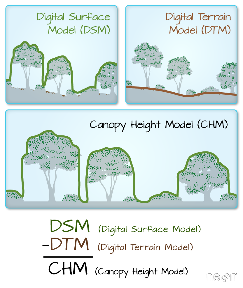
For this episode, we will be working with the Harvard Forest Digital Terrain Model data. This differs from the surface model data we’ve been working with so far in that the digital surface model (DSM) includes the tops of trees, while the digital terrain model (DTM) shows the ground level.
We’ll be looking at another model (the canopy height model) in a later episode and will see how
to calculate the CHM from the DSM and DTM. Here, we will create a map of
the Harvard Forest Digital Terrain Model (DTM_HARV) draped
or layered on top of the hillshade (DTM_hill_HARV). The
hillshade layer maps the terrain using light and shadow to create a
3D-looking image, based on a hypothetical illumination of the ground
level.
First, we need to import the DTM and DTM hillshade data.
R
DTM_HARV <-
    rast("data/NEON-DS-Airborne-Remote-Sensing/HARV/DTM/HARV_dtmCrop.tif")

DTM_hill_HARV <-
    rast("data/NEON-DS-Airborne-Remote-Sensing/HARV/DTM/HARV_DTMhill_WGS84.tif")
Next, we will convert each of these datasets to a dataframe for
plotting with ggplot.
R
DTM_HARV_df <- as.data.frame(DTM_HARV, xy = TRUE)

DTM_hill_HARV_df <- as.data.frame(DTM_hill_HARV, xy = TRUE)
Now we can create a map of the DTM layered over the hillshade.
R
ggplot() +
     geom_raster(data = DTM_HARV_df ,
                 aes(x = x, y = y,
                  fill = HARV_dtmCrop)) +
     geom_raster(data = DTM_hill_HARV_df,
                 aes(x = x, y = y,
                   alpha = HARV_DTMhill_WGS84)) +
     scale_fill_gradientn(name = "Elevation", colors = terrain.colors(10)) +
     coord_quickmap()
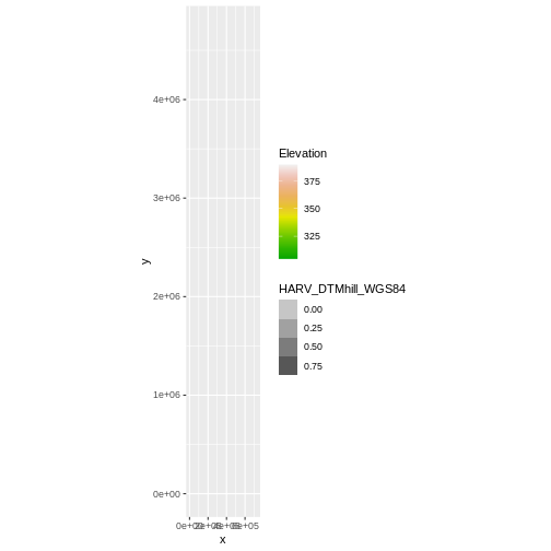
Our results are curious - neither the Digital Terrain Model
(DTM_HARV_df) nor the DTM Hillshade
(DTM_hill_HARV_df) plotted. Let’s try to plot the DTM on
its own to make sure there are data there.
R
ggplot() +
geom_raster(data = DTM_HARV_df,
    aes(x = x, y = y,
    fill = HARV_dtmCrop)) +
scale_fill_gradientn(name = "Elevation", colors = terrain.colors(10)) +
coord_quickmap()
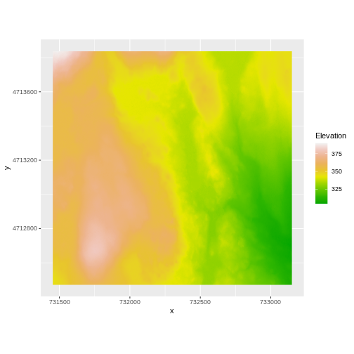
Our DTM seems to contain data and plots just fine.
Next we plot the DTM Hillshade on its own to see whether everything is OK.
R
ggplot() +
geom_raster(data = DTM_hill_HARV_df,
    aes(x = x, y = y,
    alpha = HARV_DTMhill_WGS84)) +
    coord_quickmap()
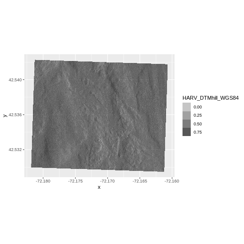
If we look at the axes, we can see that the projections of the two
rasters are different. When this is the case, ggplot won’t
render the image. It won’t even throw an error message to tell you
something has gone wrong. We can look at Coordinate Reference Systems
(CRSs) of the DTM and the hillshade data to see how they differ.
Exercise
View the CRS for each of these two datasets. What projection does each use?
R
# view crs for DTM
crs(DTM_HARV, parse = TRUE)
OUTPUT
 [1] "PROJCRS[\"WGS 84 / UTM zone 18N\","
 [2] "    BASEGEOGCRS[\"WGS 84\","
 [3] "        DATUM[\"World Geodetic System 1984\","
 [4] "            ELLIPSOID[\"WGS 84\",6378137,298.257223563,"
 [5] "                LENGTHUNIT[\"metre\",1]]],"
 [6] "        PRIMEM[\"Greenwich\",0,"
 [7] "            ANGLEUNIT[\"degree\",0.0174532925199433]],"
 [8] "        ID[\"EPSG\",4326]],"
 [9] "    CONVERSION[\"UTM zone 18N\","
[10] "        METHOD[\"Transverse Mercator\","
[11] "            ID[\"EPSG\",9807]],"
[12] "        PARAMETER[\"Latitude of natural origin\",0,"
[13] "            ANGLEUNIT[\"degree\",0.0174532925199433],"
[14] "            ID[\"EPSG\",8801]],"
[15] "        PARAMETER[\"Longitude of natural origin\",-75,"
[16] "            ANGLEUNIT[\"degree\",0.0174532925199433],"
[17] "            ID[\"EPSG\",8802]],"
[18] "        PARAMETER[\"Scale factor at natural origin\",0.9996,"
[19] "            SCALEUNIT[\"unity\",1],"
[20] "            ID[\"EPSG\",8805]],"
[21] "        PARAMETER[\"False easting\",500000,"
[22] "            LENGTHUNIT[\"metre\",1],"
[23] "            ID[\"EPSG\",8806]],"
[24] "        PARAMETER[\"False northing\",0,"
[25] "            LENGTHUNIT[\"metre\",1],"
[26] "            ID[\"EPSG\",8807]]],"
[27] "    CS[Cartesian,2],"
[28] "        AXIS[\"(E)\",east,"
[29] "            ORDER[1],"
[30] "            LENGTHUNIT[\"metre\",1]],"
[31] "        AXIS[\"(N)\",north,"
[32] "            ORDER[2],"
[33] "            LENGTHUNIT[\"metre\",1]],"
[34] "    USAGE["
[35] "        SCOPE[\"Engineering survey, topographic mapping.\"],"
[36] "        AREA[\"Between 78°W and 72°W, northern hemisphere between equator and 84°N, onshore and offshore. Bahamas. Canada - Nunavut; Ontario; Quebec. Colombia. Cuba. Ecuador. Greenland. Haiti. Jamica. Panama. Turks and Caicos Islands. United States (USA). Venezuela.\"],"
[37] "        BBOX[0,-78,84,-72]],"
[38] "    ID[\"EPSG\",32618]]"
R
# view crs for hillshade
crs(DTM_hill_HARV, parse = TRUE)
OUTPUT
 [1] "GEOGCRS[\"WGS 84\","
 [2] "    DATUM[\"World Geodetic System 1984\","
 [3] "        ELLIPSOID[\"WGS 84\",6378137,298.257223563,"
 [4] "            LENGTHUNIT[\"metre\",1]]],"
 [5] "    PRIMEM[\"Greenwich\",0,"
 [6] "        ANGLEUNIT[\"degree\",0.0174532925199433]],"
 [7] "    CS[ellipsoidal,2],"
 [8] "        AXIS[\"geodetic latitude (Lat)\",north,"
 [9] "            ORDER[1],"
[10] "            ANGLEUNIT[\"degree\",0.0174532925199433]],"
[11] "        AXIS[\"geodetic longitude (Lon)\",east,"
[12] "            ORDER[2],"
[13] "            ANGLEUNIT[\"degree\",0.0174532925199433]],"
[14] "    ID[\"EPSG\",4326]]"
DTM_HARV is in the UTM projection, with units of meters.
DTM_hill_HARV is in Geographic WGS84 - which
is represented by latitude and longitude values.
Because the two rasters are in different CRSs, they don’t line up
when plotted in R. We need to reproject (or change the projection of)
DTM_hill_HARV into the UTM CRS. Alternatively, we could
reproject DTM_HARV into WGS84.
Reproject Rasters
We can use the project() function to reproject a raster
into a new CRS. Keep in mind that reprojection only works when you first
have a defined CRS for the raster object that you want to reproject. It
cannot be used if no CRS is defined. Lucky for us, the
DTM_hill_HARV has a defined CRS.
Data Tip
When we reproject a raster, we move it from one “grid” to another. Thus, we are modifying the data! Keep this in mind as we work with raster data.
To use the project() function, we need to define two
things:
- the object we want to reproject and
- the CRS that we want to reproject it to.
The syntax is project(RasterObject, crs)
We want the CRS of our hillshade to match the DTM_HARV
raster. We can thus assign the CRS of our DTM_HARV to our
hillshade within the project() function as follows:
crs(DTM_HARV). Note that we are using the
project() function on the raster object, not the
data.frame() we use for plotting with
ggplot.
First we will reproject our DTM_hill_HARV raster data to
match the DTM_HARV raster CRS:
R
DTM_hill_UTMZ18N_HARV <- project(DTM_hill_HARV,
                                 crs(DTM_HARV))
Now we can compare the CRS of our original DTM hillshade and our new DTM hillshade, to see how they are different.
R
crs(DTM_hill_UTMZ18N_HARV, parse = TRUE)
OUTPUT
 [1] "PROJCRS[\"WGS 84 / UTM zone 18N\","
 [2] "    BASEGEOGCRS[\"WGS 84\","
 [3] "        DATUM[\"World Geodetic System 1984\","
 [4] "            ELLIPSOID[\"WGS 84\",6378137,298.257223563,"
 [5] "                LENGTHUNIT[\"metre\",1]]],"
 [6] "        PRIMEM[\"Greenwich\",0,"
 [7] "            ANGLEUNIT[\"degree\",0.0174532925199433]],"
 [8] "        ID[\"EPSG\",4326]],"
 [9] "    CONVERSION[\"UTM zone 18N\","
[10] "        METHOD[\"Transverse Mercator\","
[11] "            ID[\"EPSG\",9807]],"
[12] "        PARAMETER[\"Latitude of natural origin\",0,"
[13] "            ANGLEUNIT[\"degree\",0.0174532925199433],"
[14] "            ID[\"EPSG\",8801]],"
[15] "        PARAMETER[\"Longitude of natural origin\",-75,"
[16] "            ANGLEUNIT[\"degree\",0.0174532925199433],"
[17] "            ID[\"EPSG\",8802]],"
[18] "        PARAMETER[\"Scale factor at natural origin\",0.9996,"
[19] "            SCALEUNIT[\"unity\",1],"
[20] "            ID[\"EPSG\",8805]],"
[21] "        PARAMETER[\"False easting\",500000,"
[22] "            LENGTHUNIT[\"metre\",1],"
[23] "            ID[\"EPSG\",8806]],"
[24] "        PARAMETER[\"False northing\",0,"
[25] "            LENGTHUNIT[\"metre\",1],"
[26] "            ID[\"EPSG\",8807]]],"
[27] "    CS[Cartesian,2],"
[28] "        AXIS[\"(E)\",east,"
[29] "            ORDER[1],"
[30] "            LENGTHUNIT[\"metre\",1]],"
[31] "        AXIS[\"(N)\",north,"
[32] "            ORDER[2],"
[33] "            LENGTHUNIT[\"metre\",1]],"
[34] "    USAGE["
[35] "        SCOPE[\"Engineering survey, topographic mapping.\"],"
[36] "        AREA[\"Between 78°W and 72°W, northern hemisphere between equator and 84°N, onshore and offshore. Bahamas. Canada - Nunavut; Ontario; Quebec. Colombia. Cuba. Ecuador. Greenland. Haiti. Jamica. Panama. Turks and Caicos Islands. United States (USA). Venezuela.\"],"
[37] "        BBOX[0,-78,84,-72]],"
[38] "    ID[\"EPSG\",32618]]"
R
crs(DTM_hill_HARV, parse = TRUE)
OUTPUT
 [1] "GEOGCRS[\"WGS 84\","
 [2] "    DATUM[\"World Geodetic System 1984\","
 [3] "        ELLIPSOID[\"WGS 84\",6378137,298.257223563,"
 [4] "            LENGTHUNIT[\"metre\",1]]],"
 [5] "    PRIMEM[\"Greenwich\",0,"
 [6] "        ANGLEUNIT[\"degree\",0.0174532925199433]],"
 [7] "    CS[ellipsoidal,2],"
 [8] "        AXIS[\"geodetic latitude (Lat)\",north,"
 [9] "            ORDER[1],"
[10] "            ANGLEUNIT[\"degree\",0.0174532925199433]],"
[11] "        AXIS[\"geodetic longitude (Lon)\",east,"
[12] "            ORDER[2],"
[13] "            ANGLEUNIT[\"degree\",0.0174532925199433]],"
[14] "    ID[\"EPSG\",4326]]"
We can also compare the extent of the two objects.
R
ext(DTM_hill_UTMZ18N_HARV)
OUTPUT
SpatExtent : 731402.31567604, 733200.22199435, 4712407.19751409, 4713901.78222079 (xmin, xmax, ymin, ymax)R
ext(DTM_hill_HARV)
OUTPUT
SpatExtent : -72.1819236223343, -72.1606102223342, 42.5294079700285, 42.5423355900285 (xmin, xmax, ymin, ymax)Notice in the output above that the crs() of
DTM_hill_UTMZ18N_HARV is now UTM. However, the extent
values of DTM_hillUTMZ18N_HARV are different from
DTM_hill_HARV.
Challenge: Extent Change with CRS Change
Why do you think the two extents differ?
The extent for DTM_hill_UTMZ18N_HARV is in UTMs so the extent is in meters. The extent for DTM_hill_HARV is in lat/long so the extent is expressed in decimal degrees.
Deal with Raster Resolution
Let’s next have a look at the resolution of our reprojected hillshade versus our original data.
R
res(DTM_hill_UTMZ18N_HARV)
OUTPUT
[1] 1.001061 1.001061R
res(DTM_HARV)
OUTPUT
[1] 1 1These two resolutions are different, but they’re representing the
same data. We can tell R to force our newly reprojected raster to be 1m
x 1m resolution by adding a line of code res=1 within the
project() function. In the example below, we ensure a
resolution match by using res(DTM_HARV) as a variable.
R
  DTM_hill_UTMZ18N_HARV <- project(DTM_hill_HARV,
                                   crs(DTM_HARV),
                                   res = res(DTM_HARV))
Now both our resolutions and our CRSs match, so we can plot these two data sets together. Let’s double-check our resolution to be sure:
R
res(DTM_hill_UTMZ18N_HARV)
OUTPUT
[1] 1 1R
res(DTM_HARV)
OUTPUT
[1] 1 1For plotting with ggplot(), we will need to create a
dataframe from our newly reprojected raster.
R
DTM_hill_HARV_2_df <- as.data.frame(DTM_hill_UTMZ18N_HARV, xy = TRUE)
We can now create a plot of this data.
R
ggplot() +
     geom_raster(data = DTM_HARV_df ,
                 aes(x = x, y = y,
                  fill = HARV_dtmCrop)) +
     geom_raster(data = DTM_hill_HARV_2_df,
                 aes(x = x, y = y,
                   alpha = HARV_DTMhill_WGS84)) +
     scale_fill_gradientn(name = "Elevation", colors = terrain.colors(10)) +
     coord_quickmap()
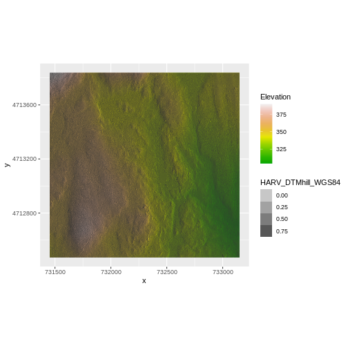
We have now successfully draped the Digital Terrain Model on top of our hillshade to produce a nice looking, textured map!
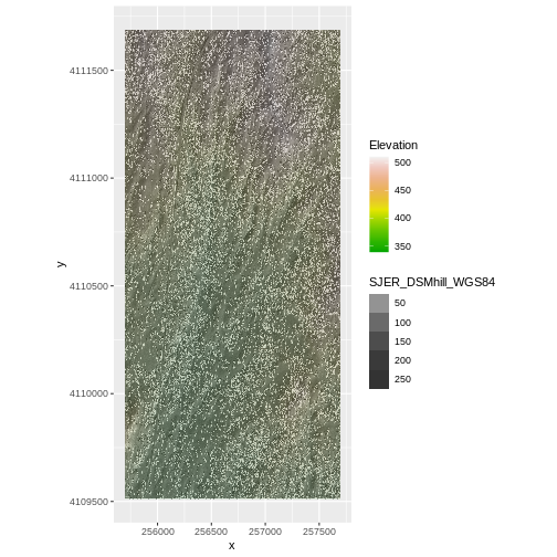
Challenge: Reproject, then Plot a Digital Terrain Model
Create a map of the San
Joaquin Experimental Range field site using the
SJER_DSMhill_WGS84.tif and SJER_dsmCrop.tif
files.
Reproject the data as necessary to make things line up!
R
# import DSM
DSM_SJER <-
    rast("data/NEON-DS-Airborne-Remote-Sensing/SJER/DSM/SJER_dsmCrop.tif")
# import DSM hillshade
DSM_hill_SJER_WGS <-
    rast("data/NEON-DS-Airborne-Remote-Sensing/SJER/DSM/SJER_DSMhill_WGS84.tif")

# reproject raster
DSM_hill_UTMZ18N_SJER <- project(DSM_hill_SJER_WGS,
                                 crs(DSM_SJER),
                                 res = 1)

# convert to data.frames
DSM_SJER_df <- as.data.frame(DSM_SJER, xy = TRUE)

DSM_hill_SJER_df <- as.data.frame(DSM_hill_UTMZ18N_SJER, xy = TRUE)

ggplot() +
     geom_raster(data = DSM_hill_SJER_df,
                 aes(x = x, y = y,
                   alpha = SJER_DSMhill_WGS84)
                 ) +
     geom_raster(data = DSM_SJER_df,
             aes(x = x, y = y,
                  fill = SJER_dsmCrop,
                  alpha=0.8)
             ) +
     scale_fill_gradientn(name = "Elevation", colors = terrain.colors(10)) +
     coord_quickmap()
Challenge: Reproject, then Plot a Digital Terrain Model (continued)
If you completed the San Joaquin plotting challenge in the Plot Raster Data in R episode, how does the map you just created compare to that map?
The maps look identical. Which is what they should be as the only difference is this one was reprojected from WGS84 to UTM prior to plotting.
Key Points
- In order to plot two raster data sets together, they must be in the same CRS.
- Use the
project()function to convert between CRSs.