Intro to Raster Data
Figure 1
Figure 2
Figure 3

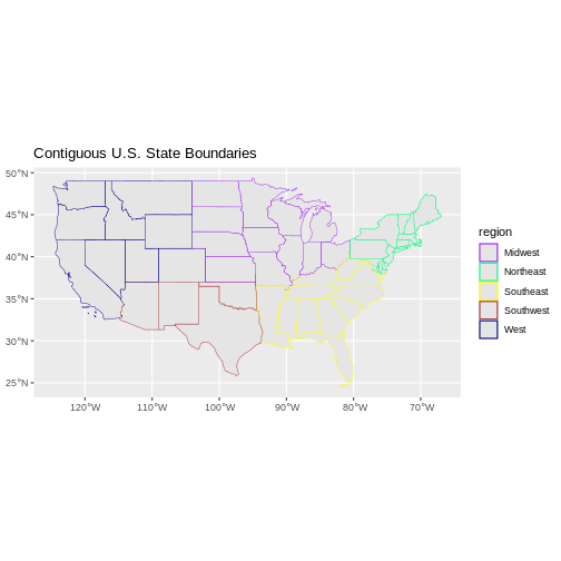
The UTM zones across the continental United
States. From: https://upload.wikimedia.org/wikipedia/commons/8/8d/Utm-zones-USA.svg
Figure 4
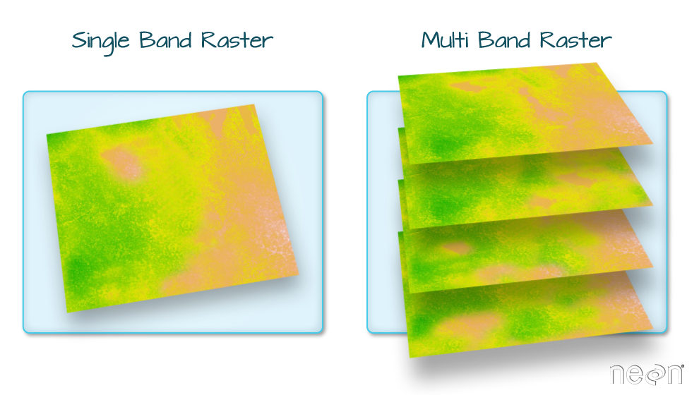
Figure 5
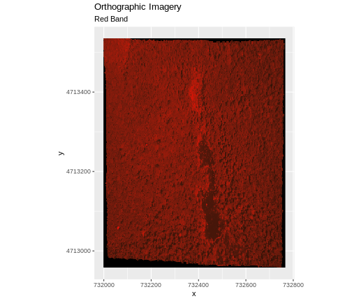
Figure 6
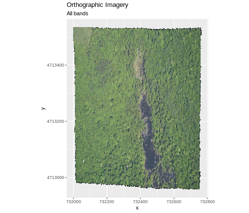
Figure 7
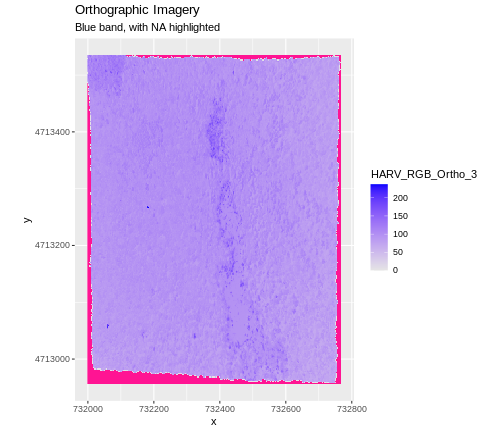
Figure 8
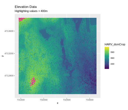
Figure 9
Figure 10
Plot Raster Data
Figure 1
Figure 2
Figure 3
Figure 4
Figure 5
Figure 6
Figure 7
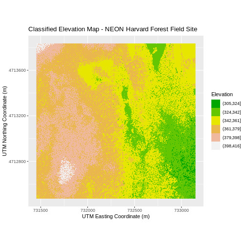
Figure 8
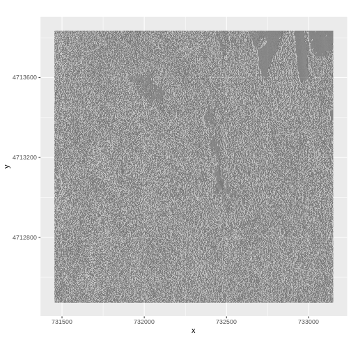
Figure 9
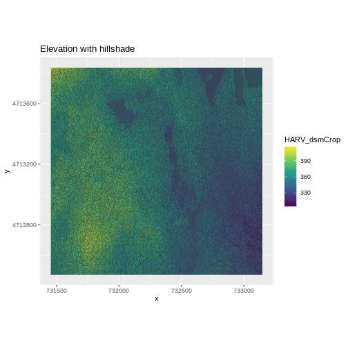
Figure 10
Figure 11
Reproject Raster Data
Figure 1
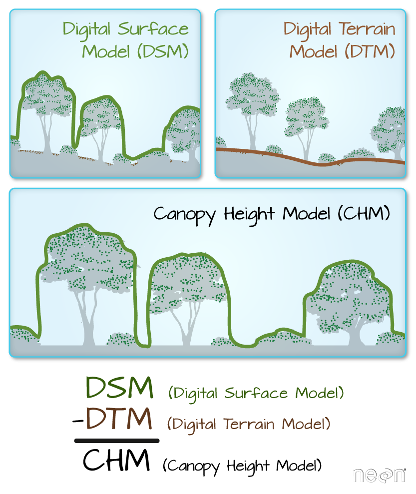
Figure 2
Figure 3

Figure 4
Figure 5
Figure 6
Raster Calculations
Figure 1
Figure 2
Figure 3
Figure 4
Figure 5
Figure 6

Figure 7
Figure 8
Figure 9

Figure 10

Figure 11
Figure 12

Figure 13
Work with Multi-Band Rasters
Figure 1
Figure 2
Figure 3
Figure 4
Figure 5
Figure 6
Figure 7
Figure 8
Figure 9
Figure 10
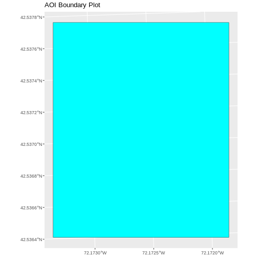
Open and Plot Vector Layers
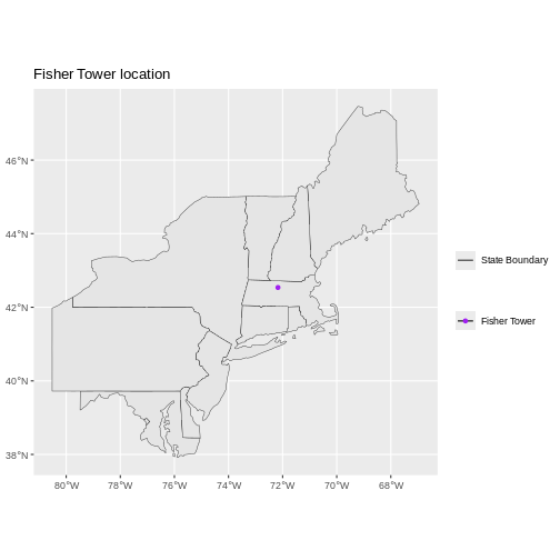
Figure 1
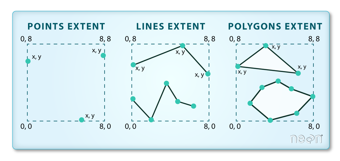
Figure 2
Explore and Plot by Vector Layer Attributes
Figure 1
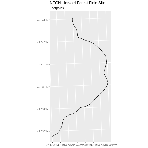
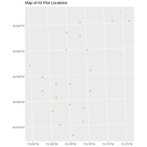
Figure 2
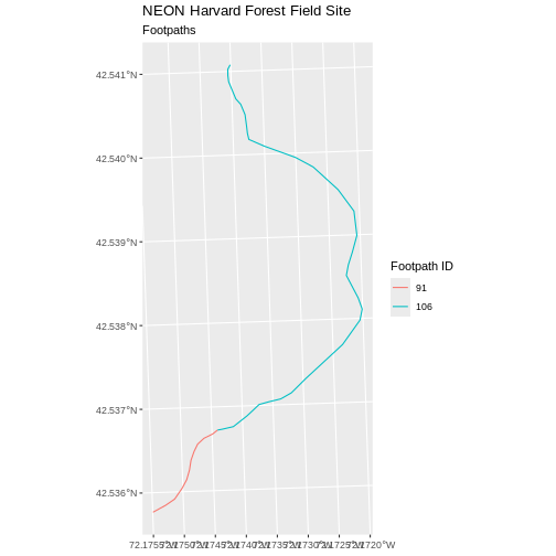
Figure 3
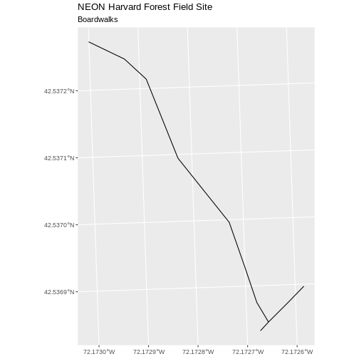
Figure 4
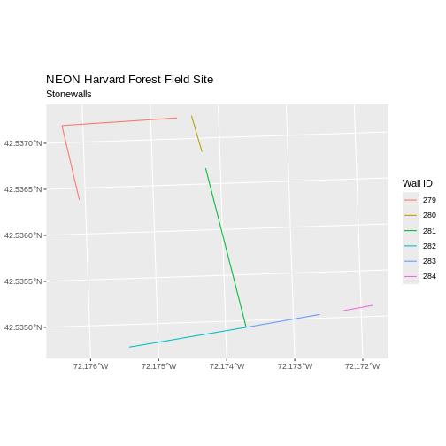
Figure 5
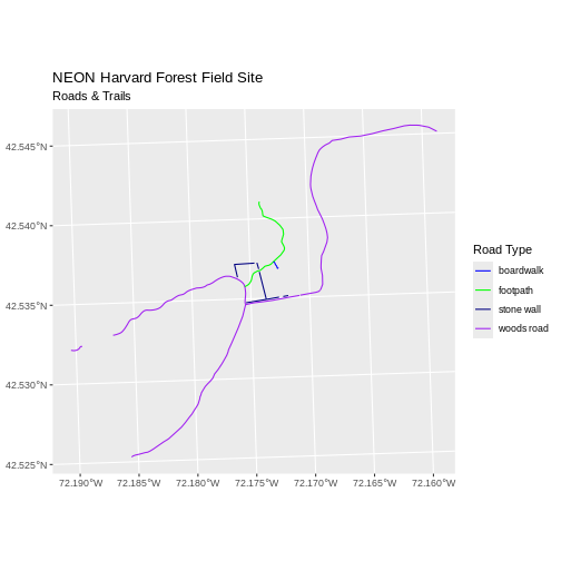
Figure 6
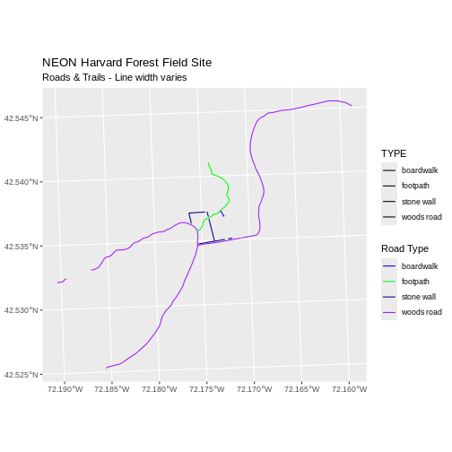
Figure 7
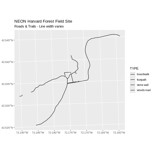
Figure 8
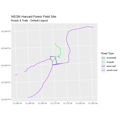
Figure 9
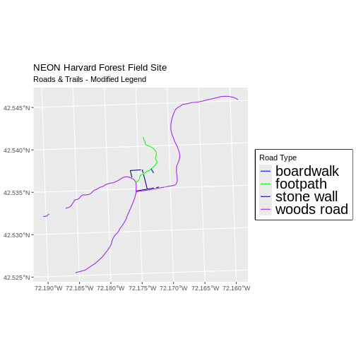
Figure 10
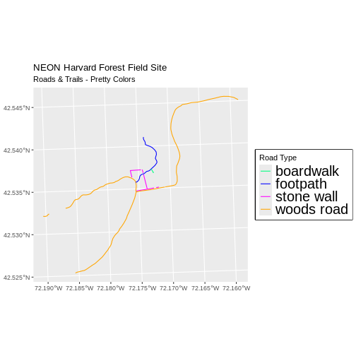
Figure 11
Figure 12
Plot Multiple Vector Layers
Figure 1
Figure 2
Figure 3

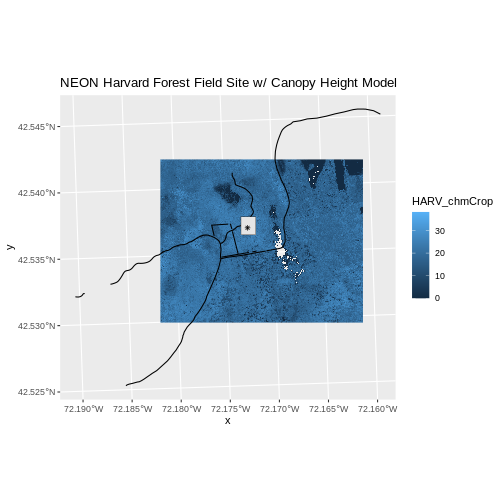
Figure 4
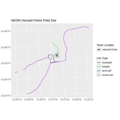
Figure 5
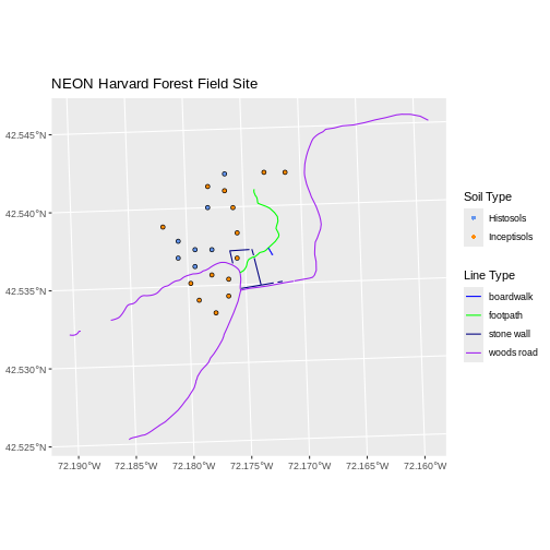
Figure 6
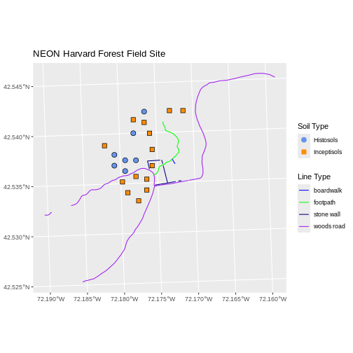
Figure 7
Handling Spatial Projection & CRS
Figure 1
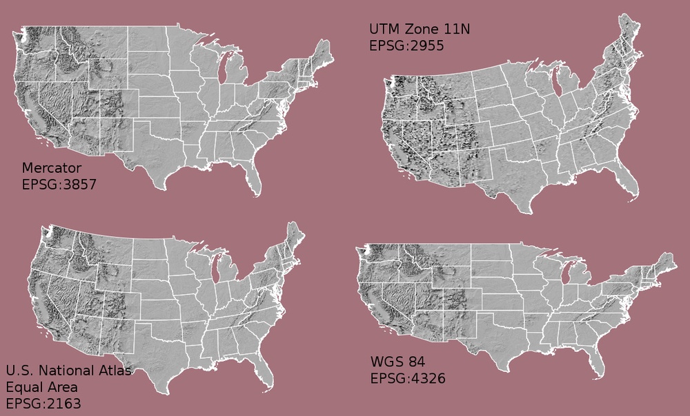 {alt=’Maps
of the United States using data in different projections.}
{alt=’Maps
of the United States using data in different projections.}
Figure 2
Figure 3
Figure 4
Figure 5
Convert from .csv to a Vector Layer
Figure 1
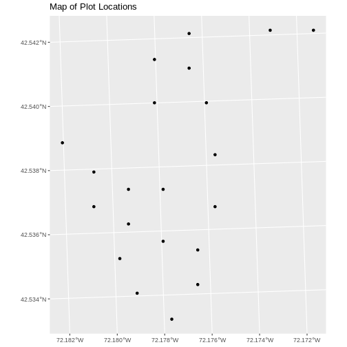
Figure 2
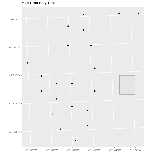
Figure 3
Manipulate Raster Data
Figure 1
Image Source: National Ecological
Observatory Network (NEON)
Figure 2

Figure 3
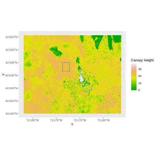
Figure 4
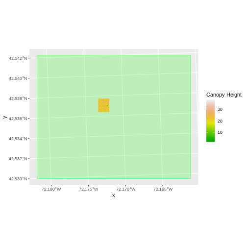
Figure 5
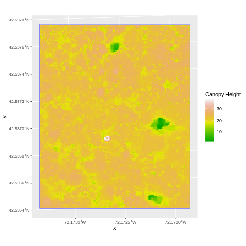
Figure 6
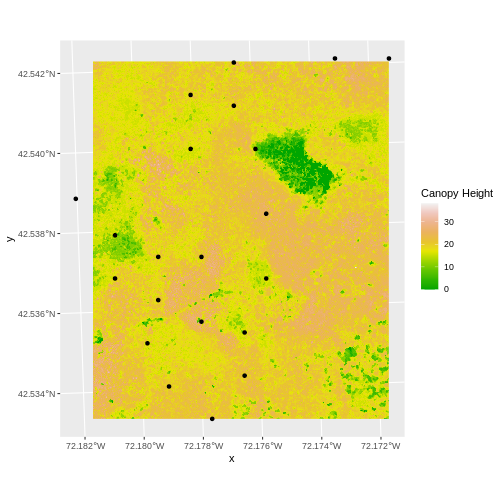
Figure 7
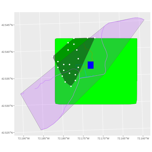
Figure 8
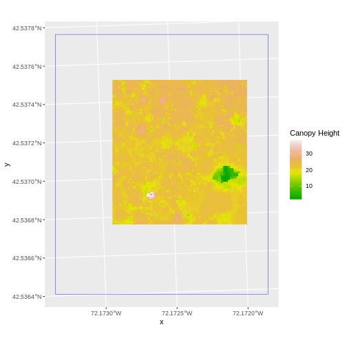
Figure 9
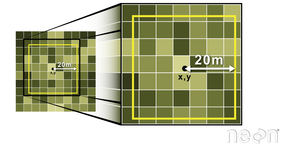 Image Source: National Ecological Observatory Network (NEON)
Figure 10
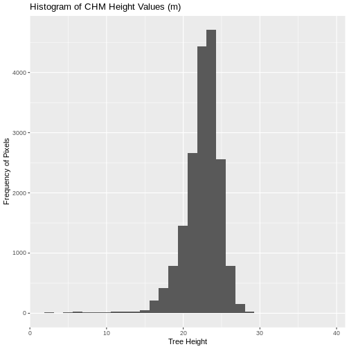
Figure 11
 Image Source: National Ecological Observatory Network (NEON)
Figure 12
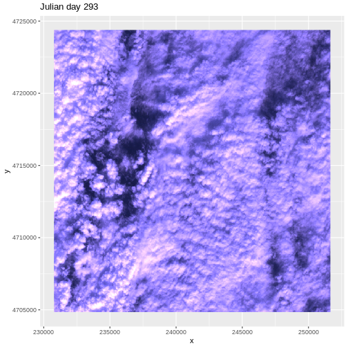
Raster Time Series Data
Figure 1
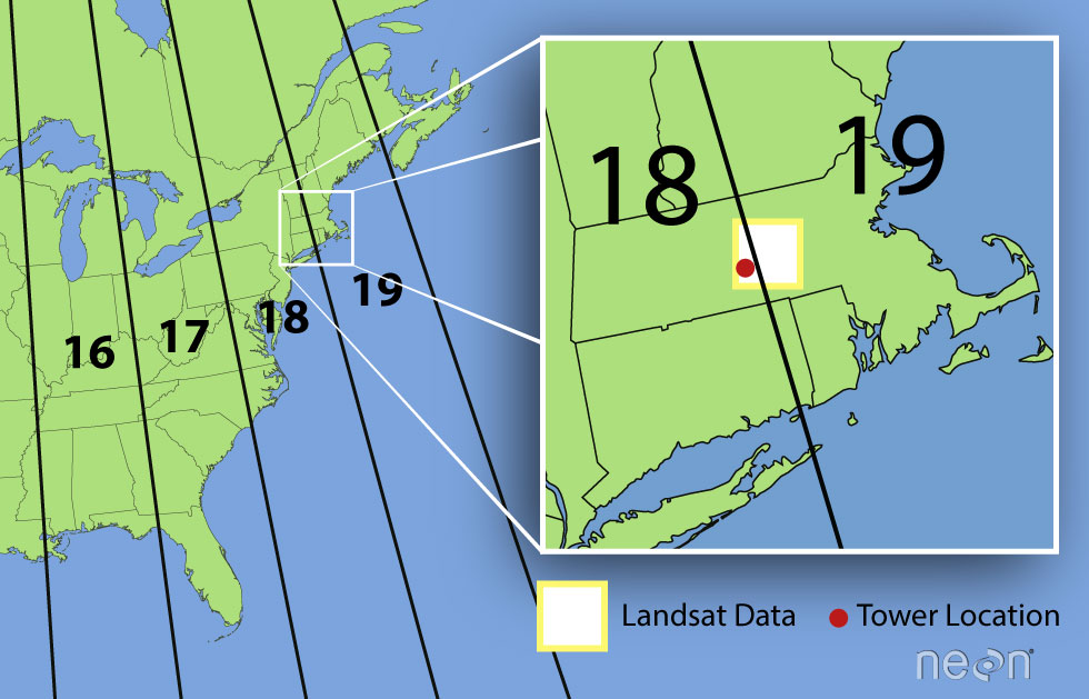
Figure 2

Figure 3
Figure 4
Figure 5
Figure 6
Figure 7
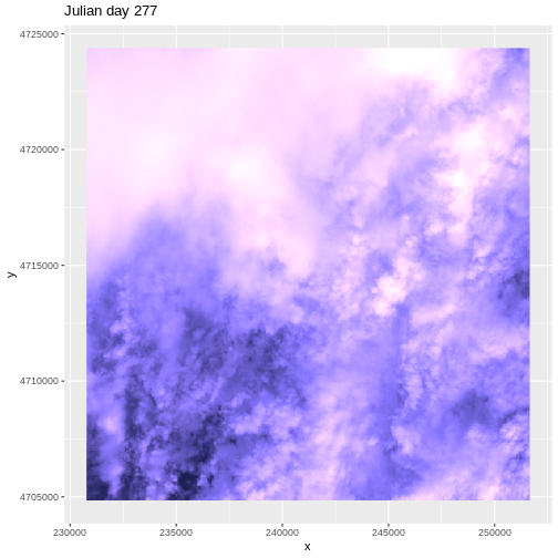
Figure 8
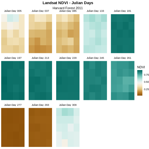
Create Publication-quality Graphics
Figure 1
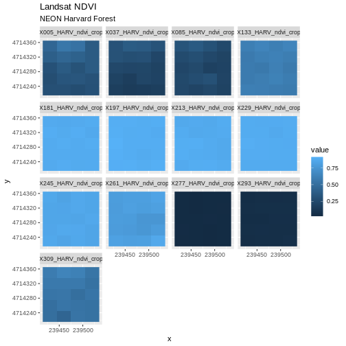
Figure 2
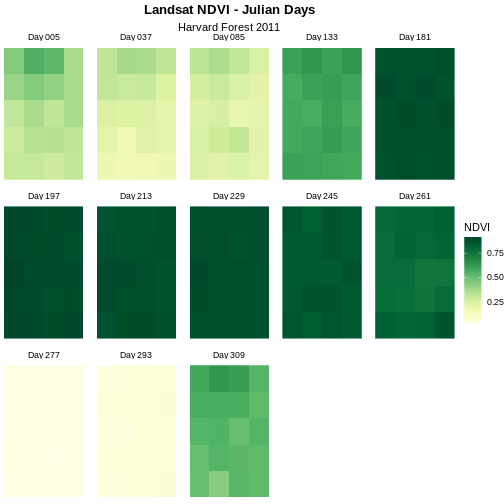
Figure 3
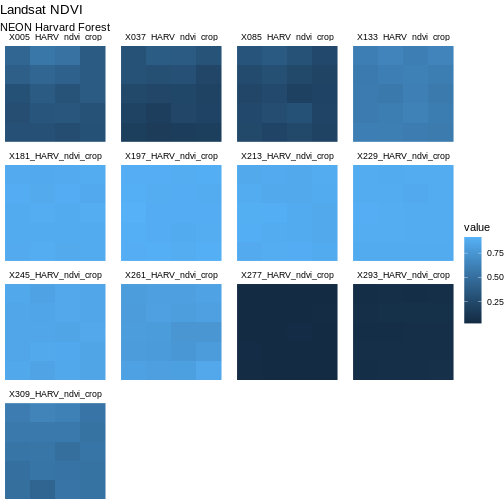
Figure 4

Figure 5

Figure 6
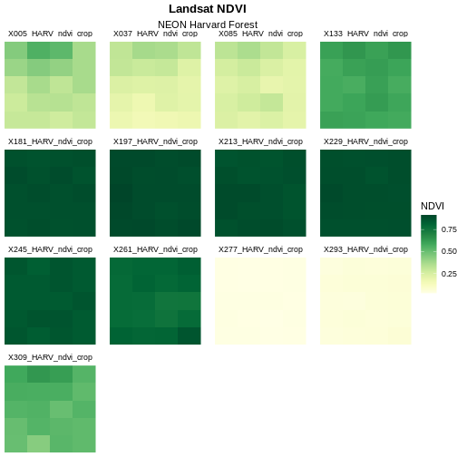
Figure 7

Figure 8
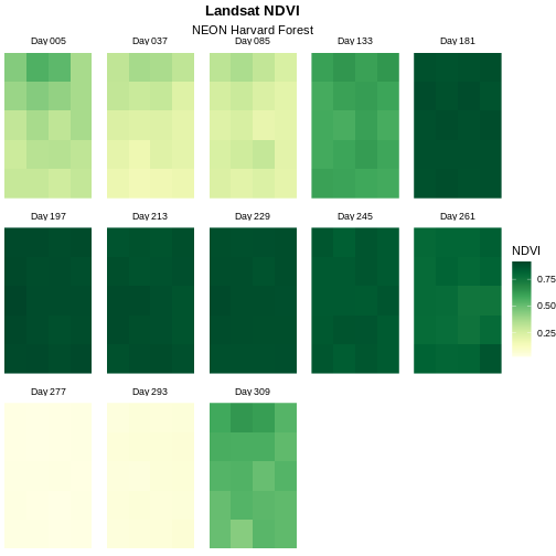
Figure 9
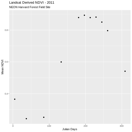
Derive Values from Raster Time Series
Figure 1
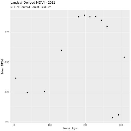
Figure 2
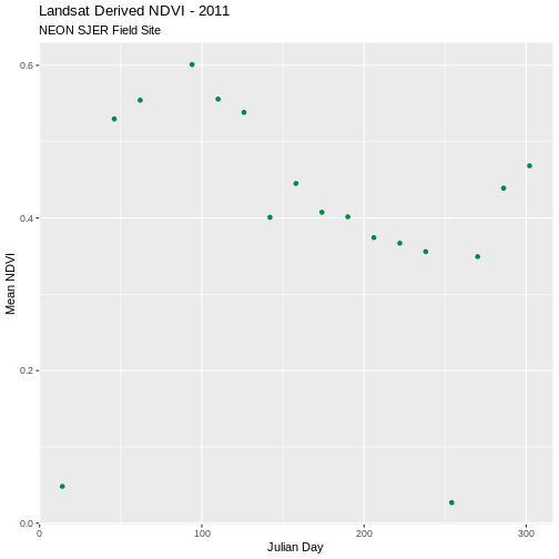
Figure 3
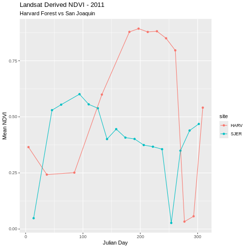
Figure 4
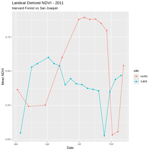
Figure 5
Figure 6