Convert from .csv to a Vector Layer
Last updated on 2024-10-15 | Edit this page
Estimated time: 60 minutes
Overview
Questions
- How can I import CSV files as vector layers in R?
Objectives
- Import .csv files containing x,y coordinate locations into R as a data frame.
- Convert a data frame to a spatial object.
- Export a spatial object to a text file.
Things You’ll Need To Complete This Episode
See the lesson homepage for detailed information about the software, data, and other prerequisites you will need to work through the examples in this episode.
This episode will review how to import spatial points stored in
.csv (Comma Separated Value) format into R as an
sf spatial object. We will also reproject data imported
from an ESRI shapefile format, export the reprojected data
as an ESRI shapefile, and plot raster and vector data as
layers in the same plot.
Spatial Data in Text Format
The HARV_PlotLocations.csv file contains
x, y (point) locations for study plot where NEON collects
data on vegetation
and other ecological metics. We would like to:
- Create a map of these plot locations.
- Export the data in an ESRI
shapefileformat to share with our colleagues. Thisshapefilecan be imported into most GIS software. - Create a map showing vegetation height with plot locations layered on top.
Spatial data are sometimes stored in a text file format
(.txt or .csv). If the text file has an
associated x and y location column, then we
can convert it into an sf spatial object. The
sf object allows us to store both the x,y
values that represent the coordinate location of each point and the
associated attribute data - or columns describing each feature in the
spatial object.
We will continue using the sf and terra
packages in this episode.
Import .csv
To begin let’s import a .csv file that contains plot
coordinate x, y locations at the NEON Harvard Forest Field
Site (HARV_PlotLocations.csv) and look at the structure of
that new object:
R
plot_locations_HARV <-
  read.csv("data/NEON-DS-Site-Layout-Files/HARV/HARV_PlotLocations.csv")

str(plot_locations_HARV)
OUTPUT
'data.frame':	21 obs. of  16 variables:
 $ easting   : num  731405 731934 731754 731724 732125 ...
 $ northing  : num  4713456 4713415 4713115 4713595 4713846 ...
 $ geodeticDa: chr  "WGS84" "WGS84" "WGS84" "WGS84" ...
 $ utmZone   : chr  "18N" "18N" "18N" "18N" ...
 $ plotID    : chr  "HARV_015" "HARV_033" "HARV_034" "HARV_035" ...
 $ stateProvi: chr  "MA" "MA" "MA" "MA" ...
 $ county    : chr  "Worcester" "Worcester" "Worcester" "Worcester" ...
 $ domainName: chr  "Northeast" "Northeast" "Northeast" "Northeast" ...
 $ domainID  : chr  "D01" "D01" "D01" "D01" ...
 $ siteID    : chr  "HARV" "HARV" "HARV" "HARV" ...
 $ plotType  : chr  "distributed" "tower" "tower" "tower" ...
 $ subtype   : chr  "basePlot" "basePlot" "basePlot" "basePlot" ...
 $ plotSize  : int  1600 1600 1600 1600 1600 1600 1600 1600 1600 1600 ...
 $ elevation : num  332 342 348 334 353 ...
 $ soilTypeOr: chr  "Inceptisols" "Inceptisols" "Inceptisols" "Histosols" ...
 $ plotdim_m : int  40 40 40 40 40 40 40 40 40 40 ...
We now have a data frame that contains 21 locations (rows) and 16
variables (attributes). Note that all of our character data was imported
into R as character (text) data. Next, let’s explore the dataframe to
determine whether it contains columns with coordinate values. If we are
lucky, our .csv will contain columns labeled:
- “X” and “Y” OR
- Latitude and Longitude OR
- easting and northing (UTM coordinates)
Let’s check out the column names of our dataframe.
R
names(plot_locations_HARV)
OUTPUT
 [1] "easting"    "northing"   "geodeticDa" "utmZone"    "plotID"
 [6] "stateProvi" "county"     "domainName" "domainID"   "siteID"
[11] "plotType"   "subtype"    "plotSize"   "elevation"  "soilTypeOr"
[16] "plotdim_m"
Identify X,Y Location Columns
Our column names include several fields that might contain spatial
information. The plot_locations_HARV$easting and
plot_locations_HARV$northing columns contain coordinate
values. We can confirm this by looking at the first six rows of our
data.
R
head(plot_locations_HARV$easting)
OUTPUT
[1] 731405.3 731934.3 731754.3 731724.3 732125.3 731634.3R
head(plot_locations_HARV$northing)
OUTPUT
[1] 4713456 4713415 4713115 4713595 4713846 4713295We have coordinate values in our data frame. In order to convert our
data frame to an sf object, we also need to know the CRS
associated with those coordinate values.
There are several ways to figure out the CRS of spatial data in text format.
- We can check the file metadata in hopes that the CRS was recorded in the data.
- We can explore the file itself to see if CRS information is embedded in the file header or somewhere in the data columns.
Following the easting and northing columns,
there is a geodeticDa and a utmZone column.
These appear to contain CRS information (datum and
projection). Let’s view those next.
R
head(plot_locations_HARV$geodeticDa)
OUTPUT
[1] "WGS84" "WGS84" "WGS84" "WGS84" "WGS84" "WGS84"R
head(plot_locations_HARV$utmZone)
OUTPUT
[1] "18N" "18N" "18N" "18N" "18N" "18N"It is not typical to store CRS information in a column. But this
particular file contains CRS information this way. The
geodeticDa and utmZone columns contain the
information that helps us determine the CRS:
-
geodeticDa: WGS84 – this is geodetic datum WGS84 -
utmZone: 18
In When Vector
Data Don’t Line Up - Handling Spatial Projection & CRS in R we
learned about the components of a proj4 string. We have
everything we need to assign a CRS to our data frame.
To create the proj4 associated with UTM Zone 18 WGS84 we
can look up the projection on the Spatial Reference
website, which contains a list of CRS formats for each projection.
From here, we can extract the proj4
string for UTM Zone 18N WGS84.
However, if we have other data in the UTM Zone 18N projection, it’s
much easier to use the st_crs() function to extract the CRS
in proj4 format from that object and assign it to our new
spatial object. We’ve seen this CRS before with our Harvard Forest study
site (point_HARV).
R
st_crs(point_HARV)
OUTPUT
Coordinate Reference System:
  User input: WGS 84 / UTM zone 18N
  wkt:
PROJCRS["WGS 84 / UTM zone 18N",
    BASEGEOGCRS["WGS 84",
        DATUM["World Geodetic System 1984",
            ELLIPSOID["WGS 84",6378137,298.257223563,
                LENGTHUNIT["metre",1]]],
        PRIMEM["Greenwich",0,
            ANGLEUNIT["degree",0.0174532925199433]],
        ID["EPSG",4326]],
    CONVERSION["UTM zone 18N",
        METHOD["Transverse Mercator",
            ID["EPSG",9807]],
        PARAMETER["Latitude of natural origin",0,
            ANGLEUNIT["Degree",0.0174532925199433],
            ID["EPSG",8801]],
        PARAMETER["Longitude of natural origin",-75,
            ANGLEUNIT["Degree",0.0174532925199433],
            ID["EPSG",8802]],
        PARAMETER["Scale factor at natural origin",0.9996,
            SCALEUNIT["unity",1],
            ID["EPSG",8805]],
        PARAMETER["False easting",500000,
            LENGTHUNIT["metre",1],
            ID["EPSG",8806]],
        PARAMETER["False northing",0,
            LENGTHUNIT["metre",1],
            ID["EPSG",8807]]],
    CS[Cartesian,2],
        AXIS["(E)",east,
            ORDER[1],
            LENGTHUNIT["metre",1]],
        AXIS["(N)",north,
            ORDER[2],
            LENGTHUNIT["metre",1]],
    ID["EPSG",32618]]
The output above shows that the points vector layer is in UTM zone
18N. We can thus use the CRS from that spatial object to convert our
non-spatial dataframe into an sf object.
Next, let’s create a crs object that we can use to
define the CRS of our sf object when we create it.
R
utm18nCRS <- st_crs(point_HARV)
utm18nCRS
OUTPUT
Coordinate Reference System:
  User input: WGS 84 / UTM zone 18N
  wkt:
PROJCRS["WGS 84 / UTM zone 18N",
    BASEGEOGCRS["WGS 84",
        DATUM["World Geodetic System 1984",
            ELLIPSOID["WGS 84",6378137,298.257223563,
                LENGTHUNIT["metre",1]]],
        PRIMEM["Greenwich",0,
            ANGLEUNIT["degree",0.0174532925199433]],
        ID["EPSG",4326]],
    CONVERSION["UTM zone 18N",
        METHOD["Transverse Mercator",
            ID["EPSG",9807]],
        PARAMETER["Latitude of natural origin",0,
            ANGLEUNIT["Degree",0.0174532925199433],
            ID["EPSG",8801]],
        PARAMETER["Longitude of natural origin",-75,
            ANGLEUNIT["Degree",0.0174532925199433],
            ID["EPSG",8802]],
        PARAMETER["Scale factor at natural origin",0.9996,
            SCALEUNIT["unity",1],
            ID["EPSG",8805]],
        PARAMETER["False easting",500000,
            LENGTHUNIT["metre",1],
            ID["EPSG",8806]],
        PARAMETER["False northing",0,
            LENGTHUNIT["metre",1],
            ID["EPSG",8807]]],
    CS[Cartesian,2],
        AXIS["(E)",east,
            ORDER[1],
            LENGTHUNIT["metre",1]],
        AXIS["(N)",north,
            ORDER[2],
            LENGTHUNIT["metre",1]],
    ID["EPSG",32618]]
R
class(utm18nCRS)
OUTPUT
[1] "crs".csv to sf object
Next, let’s convert our dataframe into an sf object. To
do this, we need to specify:
- The columns containing X (
easting) and Y (northing) coordinate values - The CRS that the column coordinate represent (units are included in
the CRS) - stored in our
utmCRSobject.
We will use the st_as_sf() function to perform the
conversion.
R
plot_locations_sp_HARV <- st_as_sf(plot_locations_HARV,
                                   coords = c("easting", "northing"),
                                   crs = utm18nCRS)
We should double check the CRS to make sure it is correct.
R
st_crs(plot_locations_sp_HARV)
OUTPUT
Coordinate Reference System:
  User input: WGS 84 / UTM zone 18N
  wkt:
PROJCRS["WGS 84 / UTM zone 18N",
    BASEGEOGCRS["WGS 84",
        DATUM["World Geodetic System 1984",
            ELLIPSOID["WGS 84",6378137,298.257223563,
                LENGTHUNIT["metre",1]]],
        PRIMEM["Greenwich",0,
            ANGLEUNIT["degree",0.0174532925199433]],
        ID["EPSG",4326]],
    CONVERSION["UTM zone 18N",
        METHOD["Transverse Mercator",
            ID["EPSG",9807]],
        PARAMETER["Latitude of natural origin",0,
            ANGLEUNIT["Degree",0.0174532925199433],
            ID["EPSG",8801]],
        PARAMETER["Longitude of natural origin",-75,
            ANGLEUNIT["Degree",0.0174532925199433],
            ID["EPSG",8802]],
        PARAMETER["Scale factor at natural origin",0.9996,
            SCALEUNIT["unity",1],
            ID["EPSG",8805]],
        PARAMETER["False easting",500000,
            LENGTHUNIT["metre",1],
            ID["EPSG",8806]],
        PARAMETER["False northing",0,
            LENGTHUNIT["metre",1],
            ID["EPSG",8807]]],
    CS[Cartesian,2],
        AXIS["(E)",east,
            ORDER[1],
            LENGTHUNIT["metre",1]],
        AXIS["(N)",north,
            ORDER[2],
            LENGTHUNIT["metre",1]],
    ID["EPSG",32618]]
Plot Spatial Object
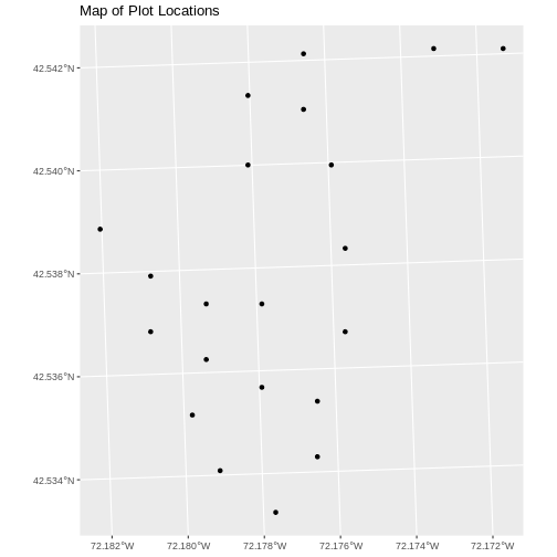
We now have a spatial R object, we can plot our newly created spatial object.
R
ggplot() +
  geom_sf(data = plot_locations_sp_HARV) +
  ggtitle("Map of Plot Locations")
Plot Extent
In Open and Plot Vector
Layers in R we learned about spatial object extent. When we plot
several spatial layers in R using ggplot, all of the layers
of the plot are considered in setting the boundaries of the plot. To
show this, let’s plot our aoi_boundary_HARV object with our
vegetation plots.
R
ggplot() +
  geom_sf(data = aoi_boundary_HARV) +
  geom_sf(data = plot_locations_sp_HARV) +
  ggtitle("AOI Boundary Plot")
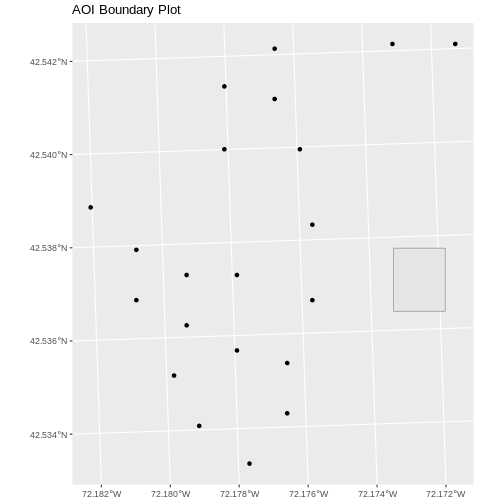
When we plot the two layers together, ggplot sets the
plot boundaries so that they are large enough to include all of the data
included in all of the layers. That’s really handy!
Challenge - Import & Plot Additional Points
We want to add two phenology plots to our existing map of vegetation plot locations.
Import the .csv: HARV/HARV_2NewPhenPlots.csv into R and
do the following:
- Find the X and Y coordinate locations. Which value is X and which value is Y?
- These data were collected in a geographic coordinate system (WGS84).
Convert the dataframe into an
sfobject. - Plot the new points with the plot location points from above. Be sure to add a legend. Use a different symbol for the 2 new points!
If you have extra time, feel free to add roads and other layers to your map!
- First we will read in the new csv file and look at the data structure.
R
newplot_locations_HARV <-
  read.csv("data/NEON-DS-Site-Layout-Files/HARV/HARV_2NewPhenPlots.csv")
str(newplot_locations_HARV)
OUTPUT
'data.frame':	2 obs. of  13 variables:
 $ decimalLat: num  42.5 42.5
 $ decimalLon: num  -72.2 -72.2
 $ country   : chr  "unitedStates" "unitedStates"
 $ stateProvi: chr  "MA" "MA"
 $ county    : chr  "Worcester" "Worcester"
 $ domainName: chr  "Northeast" "Northeast"
 $ domainID  : chr  "D01" "D01"
 $ siteID    : chr  "HARV" "HARV"
 $ plotType  : chr  "tower" "tower"
 $ subtype   : chr  "phenology" "phenology"
 $ plotSize  : int  40000 40000
 $ plotDimens: chr  "200m x 200m" "200m x 200m"
$ elevation : num 358 346- The US boundary data we worked with previously is in a geographic
WGS84 CRS. We can use that data to establish a CRS for this data. First
we will extract the CRS from the
country_boundary_USobject and confirm that it is WGS84.
R
geogCRS <- st_crs(country_boundary_US)
geogCRS
OUTPUT
Coordinate Reference System:
  User input: WGS 84
  wkt:
GEOGCRS["WGS 84",
    DATUM["World Geodetic System 1984",
        ELLIPSOID["WGS 84",6378137,298.257223563,
            LENGTHUNIT["metre",1]]],
    PRIMEM["Greenwich",0,
        ANGLEUNIT["degree",0.0174532925199433]],
    CS[ellipsoidal,2],
        AXIS["latitude",north,
            ORDER[1],
            ANGLEUNIT["degree",0.0174532925199433]],
        AXIS["longitude",east,
            ORDER[2],
            ANGLEUNIT["degree",0.0174532925199433]],
    ID["EPSG",4326]]
Then we will convert our new data to a spatial dataframe, using the
geogCRS object as our CRS.
R
newPlot.Sp.HARV <- st_as_sf(newplot_locations_HARV,
                            coords = c("decimalLon", "decimalLat"),
                            crs = geogCRS)
Next we’ll confirm that the CRS for our new object is correct.
R
st_crs(newPlot.Sp.HARV)
OUTPUT
Coordinate Reference System:
User input: WGS 84
wkt:
GEOGCRS["WGS 84",
DATUM["World Geodetic System 1984",
ELLIPSOID["WGS 84",6378137,298.257223563,
LENGTHUNIT["metre",1]]],
PRIMEM["Greenwich",0,
ANGLEUNIT["degree",0.0174532925199433]],
CS[ellipsoidal,2],
AXIS["latitude",north,
ORDER[1],
ANGLEUNIT["degree",0.0174532925199433]],
AXIS["longitude",east,
ORDER[2],
ANGLEUNIT["degree",0.0174532925199433]],
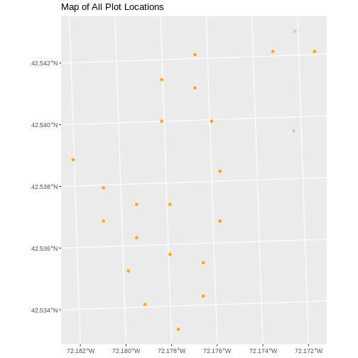
ID["EPSG",4326]]We will be adding these new data points to the plot we created
before. The data for the earlier plot was in UTM. Since we’re using
ggplot, it will reproject the data for us.
- Now we can create our plot.
R
ggplot() +
  geom_sf(data = plot_locations_sp_HARV, color = "orange") +
  geom_sf(data = newPlot.Sp.HARV, color = "lightblue") +
  ggtitle("Map of All Plot Locations")
Export to an ESRI shapefile
We can write an R spatial object to an ESRI shapefile
using the st_write function in sf. To do this
we need the following arguments:
- the name of the spatial object
(
plot_locations_sp_HARV) - the directory where we want to save our ESRI
shapefile(to usecurrent = getwd()or you can specify a different path) - the name of the new ESRI
shapefile(PlotLocations_HARV) - the driver which specifies the file format (ESRI Shapefile)
We can now export the spatial object as an ESRI
shapefile.
R
st_write(plot_locations_sp_HARV,
         "data/PlotLocations_HARV.shp", driver = "ESRI Shapefile")
Key Points
- Know the projection (if any) of your point data prior to converting to a spatial object.
- Convert a data frame to an
sfobject using thest_as_sf()function. - Export an
sfobject as text using thest_write()function.