Content from Introduction to R and RStudio

---

Last updated on 2024-03-12 | Edit this page

Overview

Questions

• How to find your way around RStudio?
• How to interact with R?
• How to install packages?

Objectives

• Describe the purpose and use of each pane in the RStudio IDE
• Locate buttons and options in the RStudio IDE
• Define a variable
• Assign data to a variable
• Use mathematical and comparison operators
• Call functions
• Manage packages

Motivation

---

Science is a multi-step process: once you’ve designed an experiment and collected data, the real fun begins! This lesson will teach you how to start this process using R and RStudio. We will begin with raw data, perform exploratory analyses, and learn how to plot results graphically. This example starts with a dataset from gapminder.org containing population information for many countries through time. Can you read the data into R? Can you plot the population for Senegal? Can you calculate the average income for countries on the continent of Asia? By the end of these lessons you will be able to do things like plot the populations for all of these countries in under a minute!

Before Starting The Workshop

---

Please ensure you have the latest version of R and RStudio installed on your machine. This is important, as some packages used in the workshop may not install correctly (or at all) if R is not up to date.

• Download and install the latest version of R here
• Download and install RStudio here

Introduction to RStudio

---

Throughout this lesson, we’re going to teach you some of the fundamentals of the R language as well as some best practices for organizing code for scientific projects that will make your life easier.

We’ll be using RStudio: a free, open source R integrated development environment (IDE). It provides a built in editor, works on all platforms (including on servers) and provides many advantages such as integration with version control and project management.

Basic layout

When you first open RStudio, you will be greeted by three panels:

• The interactive R console (entire left)
• Environment/History (tabbed in upper right)
• Files/Plots/Packages/Help/Viewer (tabbed in lower right)

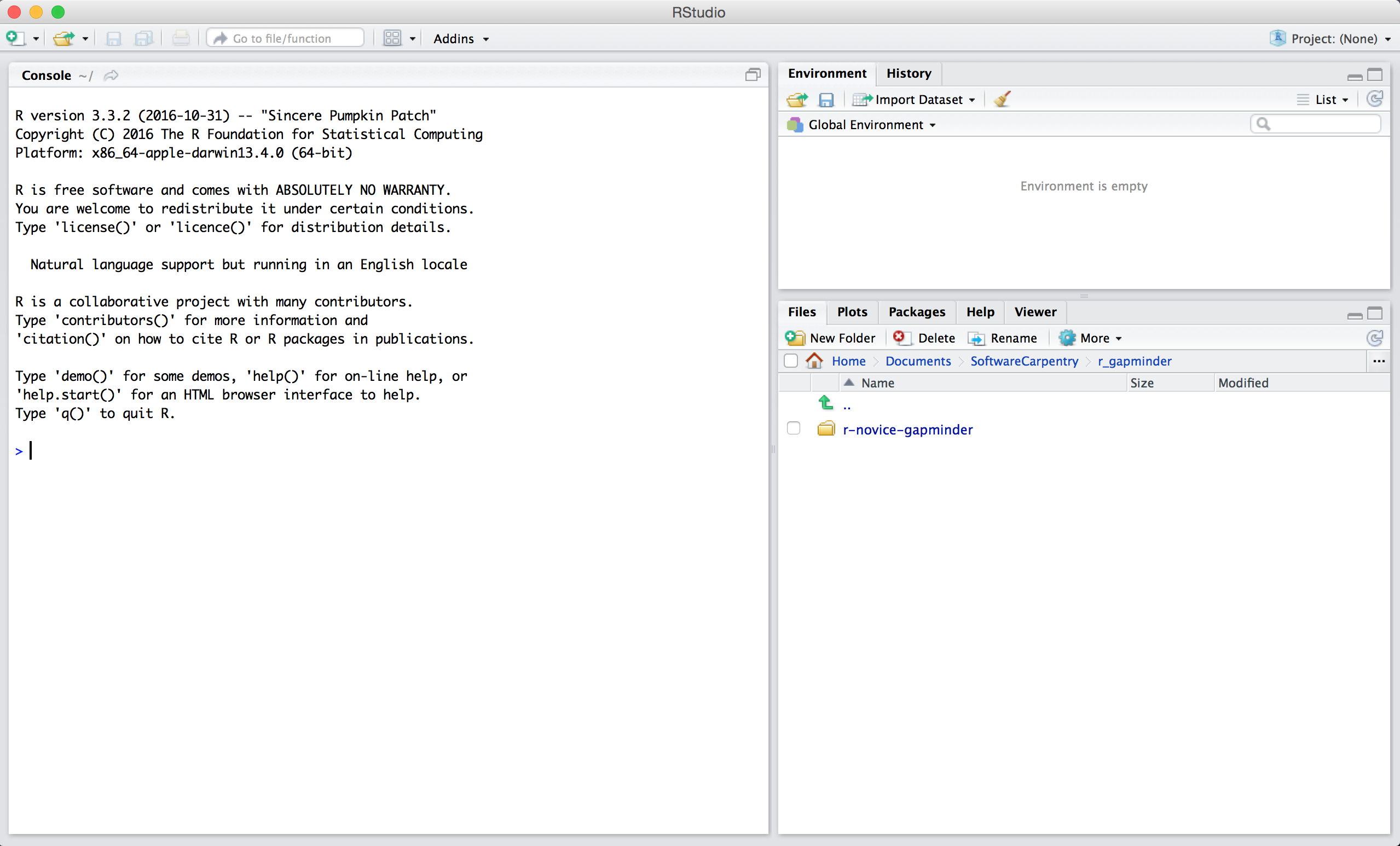
Once you open files, such as R scripts, an editor panel will also open in the top left.

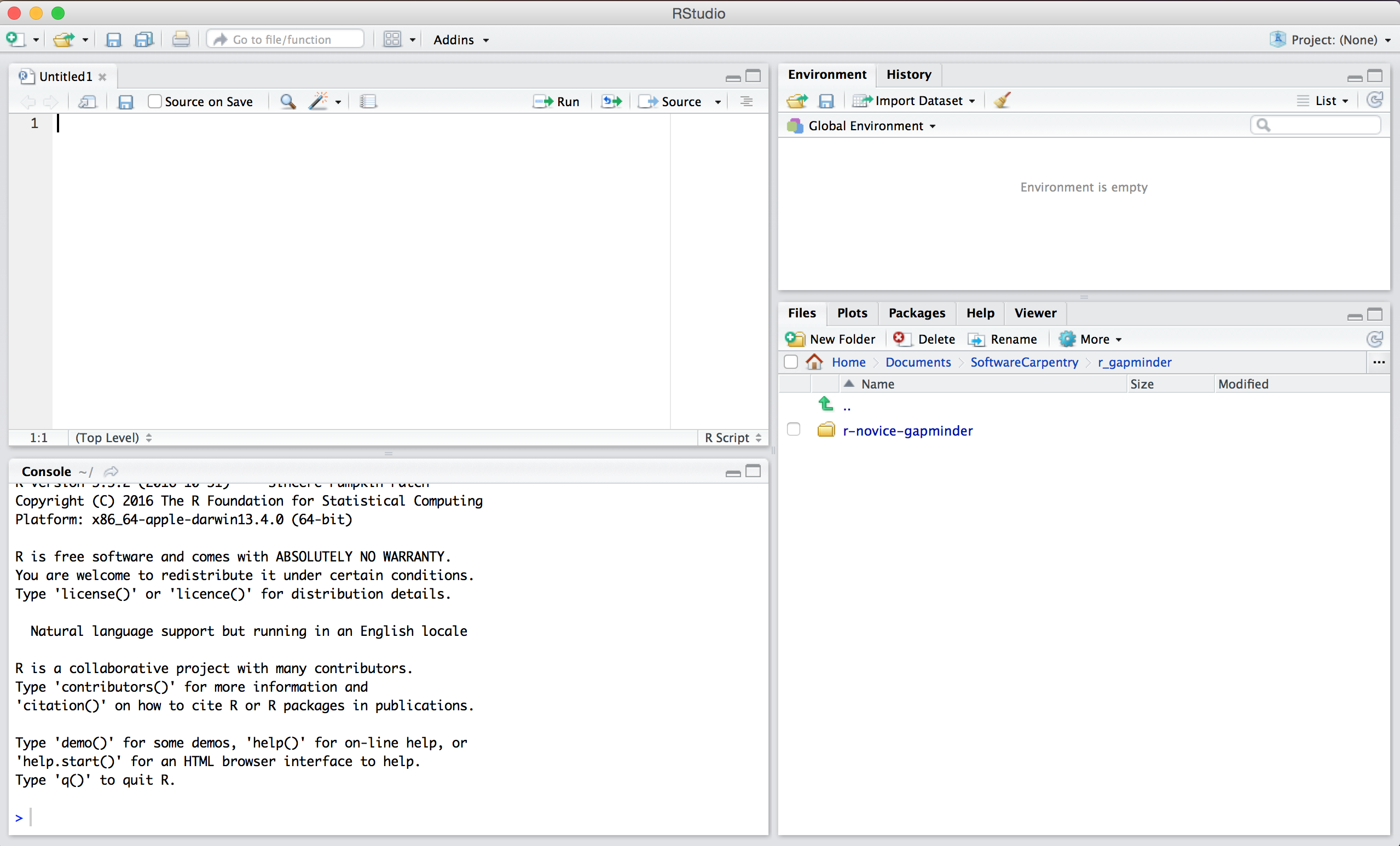
Workflow within RStudio

---

There are two main ways one can work within RStudio.

1. Test and play within the interactive R console then copy code into a .R file to run later.

• This works well when doing small tests and initially starting off.
• It quickly becomes laborious

2. Start writing in an .R file and use RStudio’s shortcut keys for the Run command to push the current line, selected lines or modified lines to the interactive R console.

• This is a great way to start; all your code is saved for later
• You will be able to run the file you create from within RStudio or using R’s source() function.

Tip: Running segments of your code

RStudio offers you great flexibility in running code from within the editor window. There are buttons, menu choices, and keyboard shortcuts. To run the current line, you can

1. click on the Run button above the editor panel, or
2. select “Run Lines” from the “Code” menu, or
3. hit Ctrl+Enter in Windows, Ctrl+Return in Linux, or ⌘+Return on OS X. (This shortcut can also be seen by hovering the mouse over the button). To run a block of code, select it and then Run. If you have modified a line of code within a block of code you have just run, there is no need to reselect the section and Run, you can use the next button along, Re-run the previous region. This will run the previous code block including the modifications you have made.

Introduction to R

---

Much of your time in R will be spent in the R interactive console. This is where you will run all of your code, and can be a useful environment to try out ideas before adding them to an R script file. This console in RStudio is the same as the one you would get if you typed in R in your command-line environment.

The first thing you will see in the R interactive session is a bunch of information, followed by a “>” and a blinking cursor. When you are running a section of your code, this is the location where R will first read your code, attempt to execute them, and then returns a result.

Using R as a calculator

---

The simplest thing you could do with R is do arithmetic:

R

1 + 100

OUTPUT

[1] 101

And R will print out the answer, with a preceding “[1]”. Don’t worry about this for now, we’ll explain that later. For now think of it as indicating output.

Like bash, if you type in an incomplete command, R will wait for you to complete it:

R

> 1 +

OUTPUT

+

Any time you hit return and the R session shows a “+” instead of a “>”, it means it’s waiting for you to complete the command. If you want to cancel a command you can simply hit “Esc” and RStudio will give you back the “>” prompt.

Tip: Cancelling commands

If you’re using R from the command line instead of from within RStudio, you need to use Ctrl+C instead of Esc to cancel the command. This applies to Mac users as well!

Cancelling a command isn’t only useful for killing incomplete commands: you can also use it to tell R to stop running code (for example if it’s taking much longer than you expect), or to get rid of the code you’re currently writing.

When using R as a calculator, the order of operations is the same as you would have learned back in school.

From highest to lowest precedence:

• Parentheses: (, )
• Exponents: ^ or **
• Divide: /
• Multiply: *
• Add: +
• Subtract: -

R

3 + 5 * 2

OUTPUT

[1] 13

Use parentheses to group operations in order to force the order of evaluation if it differs from the default, or to make clear what you intend.

R

(3 + 5) * 2

OUTPUT

[1] 16

This can get unwieldy when not needed, but clarifies your intentions. Remember that others may later read your code.

R

(3 + (5 * (2 ^ 2))) # hard to read
3 + 5 * 2 ^ 2       # clear, if you remember the rules
3 + 5 * (2 ^ 2)     # if you forget some rules, this might help

The text after each line of code is called a “comment”. Anything that follows after the hash (or octothorpe) symbol # is ignored by R when it executes code.

Really small or large numbers get a scientific notation:

R

2/10000

OUTPUT

[1] 2e-04

Which is shorthand for “multiplied by 10^XX”. So 2e-4 is shorthand for 2 * 10^(-4).

You can write numbers in scientific notation too:

R

5e3  # Note the lack of minus here

OUTPUT

[1] 5000

Don’t worry about trying to remember every function in R. You can look them up using a search engine, or if you can remember the start of the function’s name, use the tab completion in RStudio.

This is one advantage that RStudio has over R on its own, it has auto-completion abilities that allow you to more easily look up functions, their arguments, and the values that they take.

Typing a ? before the name of a command will open the help page for that command. As well as providing a detailed description of the command and how it works, scrolling to the bottom of the help page will usually show a collection of code examples which illustrate command usage. We’ll go through an example later.

Comparing things

---

We can also do comparison in R:

R

1 == 1  # equality (note two equals signs, read as "is equal to")

OUTPUT

[1] TRUE

R

1 != 2  # inequality (read as "is not equal to")

OUTPUT

[1] TRUE

R

1 < 2  # less than

OUTPUT

[1] TRUE

R

1 <= 1  # less than or equal to

OUTPUT

[1] TRUE

R

1 > 0  # greater than

OUTPUT

[1] TRUE

R

1 >= -9 # greater than or equal to

OUTPUT

[1] TRUE

Tip: Comparing Numbers

A word of warning about comparing numbers: you should never use == to compare two numbers unless they are integers (a data type which can specifically represent only whole numbers).

Computers may only represent decimal numbers with a certain degree of precision, so two numbers which look the same when printed out by R, may actually have different underlying representations and therefore be different by a small margin of error (called Machine numeric tolerance).

Instead you should use the all.equal function.

Further reading: http://floating-point-gui.de/

Variables and assignment

---

We can store values in variables using the assignment operator <-, like this:

R

x <- 1/40

Notice that assignment does not print a value. Instead, we stored it for later in something called a variable. x now contains the value 0.025:

R

x

OUTPUT

[1] 0.025

More precisely, the stored value is a decimal approximation of this fraction called a floating point number.

Look for the Environment tab in one of the panes of RStudio, and you will see that x and its value have appeared. Our variable x can be used in place of a number in any calculation that expects a number:

R

log(x)

OUTPUT

[1] -3.688879

Notice also that variables can be reassigned:

R

x <- 100

x used to contain the value 0.025 and and now it has the value 100.

Assignment values can contain the variable being assigned to:

R

x <- x + 1 #notice how RStudio updates its description of x on the top right tab
y <- x * 2

The right hand side of the assignment can be any valid R expression. The right hand side is fully evaluated before the assignment occurs.

Challenge 1

What will be the value of each variable after each statement in the following program?

R

mass <- 47.5
age <- 122
mass <- mass * 2.3
age <- age - 20

Solution to challenge 1

R

mass <- 47.5

This will give a value of 47.5 for the variable mass

R

age <- 122

This will give a value of 122 for the variable age

R

mass <- mass * 2.3

This will multiply the existing value of 47.5 by 2.3 to give a new value of 109.25 to the variable mass.

R

age <- age - 20

This will subtract 20 from the existing value of 122 to give a new value of 102 to the variable age.

Challenge 2

Run the code from the previous challenge, and write a command to compare mass to age. Is mass larger than age?

Solution to challenge 2

One way of answering this question in R is to use the > to set up the following:

R

mass > age

OUTPUT

[1] TRUE

This should yield a boolean value of TRUE since 109.25 is greater than 102.

Variable names can contain letters, numbers, underscores and periods. They cannot start with a number nor contain spaces at all. Different people use different conventions for long variable names, these include

• periods.between.words
• underscores_between_words
• camelCaseToSeparateWords

What you use is up to you, but be consistent.

It is also possible to use the = operator for assignment:

R

x = 1/40

But this is much less common among R users. The most important thing is to be consistent with the operator you use. There are occasionally places where it is less confusing to use <- than =, and it is the most common symbol used in the community. So the recommendation is to use <-.

Challenge 3

Which of the following are valid R variable names?

R

min_height
max.height
_age
.mass
MaxLength
min-length
2widths
celsius2kelvin

Solution to challenge 3

The following can be used as R variables:

R

min_height
max.height
MaxLength
celsius2kelvin

The following creates a hidden variable:

R

.mass

We won’t be discussing hidden variables in this lesson. We recommend not using a period at the beginning of variable names unless you intend your variables to be hidden.

The following will not be able to be used to create a variable

R

_age
min-length
2widths

Installing Packages

---

We can use R as a calculator to do mathematical operations (e.g., addition, subtraction, multiplication, division), as we did above. However, we can also use R to carry out more complicated analyses, make visualizations, and much more. In later episodes, we’ll use R to do some data wrangling, plotting, and saving of reformatted data.

R coders around the world have developed collections of R code to accomplish themed tasks (e.g., data wrangling). These collections of R code are known as R packages. It is also important to note that R packages refer to code that is not automatically downloaded when we install R on our computer. Therefore, we’ll have to install each R package that we want to use (more on this below).

We will practice using the dplyr package to wrangle our datasets in episode 6 and will also practice using the ggplot2 package to plot our data in episode 7. To give an example, the dplyr package includes code for a function called filter(). A function is something that takes input(s) does some internal operations and produces output(s). For the filter() function, the inputs are a dataset and a logical statement (i.e., when data value is greater than or equal to 100) and the output is data within the dataset that has a value greater than or equal to 100.

There are two main ways to install packages in R:

1. If you are using RStudio, we can go to Tools > Install Packages... and then search for the name of the R package we need and click Install.

2. We can use the install.packages( ) function. We can do this to install the dplyr R package.

R

install.packages("dplyr")

OUTPUT

The following package(s) will be installed:
- dplyr [1.1.4]
- vctrs [0.6.5]
These packages will be installed into "~/work/r-intro-geospatial/r-intro-geospatial/renv/profiles/lesson-requirements/renv/library/R-4.3/x86_64-pc-linux-gnu".

# Installing packages --------------------------------------------------------
- Installing vctrs ...                          OK [linked from cache]
- Installing dplyr ...                          OK [linked from cache]
Successfully installed 2 packages in 9.1 milliseconds.

It’s important to note that we only need to install the R package on our computer once. Well, if we install a new version of R on the same computer, then we will likely need to also re-install the R packages too.

Challenge 4

What code would we use to install the ggplot2 package?

Solution to challenge 4

We would use the following R code to install the ggplot2 package:

R

install.packages("ggplot2")

Now that we’ve installed the R package, we’re ready to use it! To use the R package, we need to “load” it into our R session. We can think of “loading” an R packages as telling R that we’re ready to use the package we just installed. It’s important to note that while we only have to install the package once, we’ll have to load the package each time we open R (or RStudio).

To load an R package, we use the library( ) function. We can load the dplyr package like this:

R

library(dplyr)

OUTPUT

Attaching package: 'dplyr'

OUTPUT

The following objects are masked from 'package:stats':

    filter, lag

OUTPUT

The following objects are masked from 'package:base':

    intersect, setdiff, setequal, union

Challenge 5

Which of the following could we use to load the ggplot2 package? (Select all that apply.)

1. install.packages(“ggplot2”)
2. library(“ggplot2”)
3. library(ggplot2)
4. library(ggplo2)

Solution to challenge 5

The correct answers are b and c. Answer a will install, not load, the ggplot2 package. Answer b will correctly load the ggplot2 package. Note there are no quotation marks. Answer c will correctly load the ggplot2 package. Note there are quotation marks. Answer d will produce an error because ggplot2 is misspelled.

Note: It is more common for coders to not use quotation marks when loading an R package (i.e., answer c).

R

library(ggplot2)

Key Points

• Use RStudio to write and run R programs.
• R has the usual arithmetic operators.
• Use <- to assign values to variables.
• Use install.packages() to install packages (libraries).

Content from Project Management With RStudio

---

Last updated on 2024-03-12 | Edit this page

Overview

Questions

• How can I manage my projects in R?

Objectives

• Create self-contained projects in RStudio

Introduction

---

The scientific process is naturally incremental, and many projects start life as random notes, some code, then a manuscript, and eventually everything is a bit mixed together. Organising a project involving spatial data is no different from any other data analysis project, although you may require more disk space than usual.

Managing your projects in a reproducible fashion doesn’t just make your science reproducible, it makes your life easier.

— Vince Buffalo (@vsbuffalo) April 15, 2013

Most people tend to organize their projects like this:

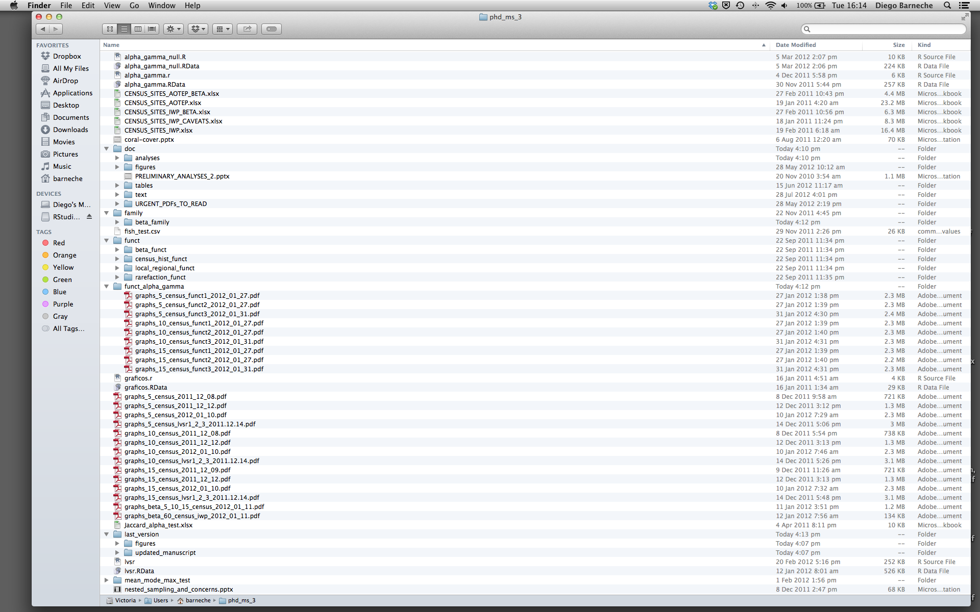
There are many reasons why we should ALWAYS avoid this:

1. It is really hard to tell which version of your data is the original and which is the modified;
2. It gets really messy because it mixes files with various extensions together;
3. It probably takes you a lot of time to actually find things, and relate the correct figures to the exact code that has been used to generate it;

A good project layout will ultimately make your life easier:

• It will help ensure the integrity of your data;
• It makes it simpler to share your code with someone else (a lab-mate, collaborator, or supervisor);
• It allows you to easily upload your code with your manuscript submission;
• It makes it easier to pick the project back up after a break.

A possible solution

---

Fortunately, there are tools and packages which can help you manage your work effectively.

One of the most powerful and useful aspects of RStudio is its project management functionality. We’ll be using this today to create a self-contained, reproducible project.

Challenge: Creating a self-contained project

We’re going to create a new project in RStudio:

1. Click the “File” menu button, then “New Project”.
2. Click “New Directory”.
3. Click “Empty Project”.
4. Type in “r-geospatial” as the name of the directory.
5. Click the “Create Project” button.

A key advantage of an RStudio Project is that whenever we open this project in subsequent RStudio sessions our working directory will always be set to the folder r-geospatial. Let’s check our working directory by entering the following into the R console:

R

getwd()

R should return your/path/r-geospatial as the working directory.

Best practices for project organization

---

Although there is no “best” way to lay out a project, there are some general principles to adhere to that will make project management easier:

Treat data as read only

This is probably the most important goal of setting up a project. Data is typically time consuming and/or expensive to collect. Working with them interactively (e.g., in Excel) where they can be modified means you are never sure of where the data came from, or how it has been modified since collection. It is therefore a good idea to treat your data as “read-only”.

Data Cleaning

In many cases your data will be “dirty”: it will need significant preprocessing to get into a format R (or any other programming language) will find useful. This task is sometimes called “data munging”. I find it useful to store these scripts in a separate folder, and create a second “read-only” data folder to hold the “cleaned” data sets.

Treat generated output as disposable

Anything generated by your scripts should be treated as disposable: it should all be able to be regenerated from your scripts.

There are lots of different ways to manage this output. I find it useful to have an output folder with different sub-directories for each separate analysis. This makes it easier later, as many of my analyses are exploratory and don’t end up being used in the final project, and some of the analyses get shared between projects.

Keep related data together

Some GIS file formats are really 3-6 files that need to be kept together and have the same name, e.g. shapefiles. It may be tempting to store those components separately, but your spatial data will be unusable if you do that.

Keep a consistent naming scheme

It is generally best to avoid renaming downloaded spatial data, so that a clear connection is maintained with the point of truth. You may otherwise find yourself wondering whether file_A really is just a copy of Official_file_on_website or not.

For datasets you generate, it’s worth taking the time to come up with a naming convention that works for your project, and sticking to it. File names don’t have to be long, they just have to be long enough that you can tell what the file is about. Date generated, topic, and whether a product is intermediate or final are good bits of information to keep in a file name. For more tips on naming files, check out the slides from Jenny Bryan’s talk “Naming things” at the 2015 Reproducible Science Workshop.

Tip: Good Enough Practices for Scientific Computing

Good Enough Practices for Scientific Computing gives the following recommendations for project organization:

1. Put each project in its own directory, which is named after the project.
2. Put text documents associated with the project in the doc directory.
3. Put raw data and metadata in the data directory, and files generated during cleanup and analysis in a results directory.
4. Put source for the project’s scripts and programs in the src directory, and programs brought in from elsewhere or compiled locally in the bin directory.
5. Name all files to reflect their content or function.

Save the data in the data directory

Now we have a good directory structure we will now place/save our data files in the data/ directory.

Challenge 1

1. Download each of the data files listed below (Ctrl+S, right mouse click -> “Save as”, or File -> “Save page as”)

• nordic country data
• nordic country data (version 2)
• gapminder data

2. Make sure the files have the following names:

• nordic-data.csv
• nordic-data-2.csv
• gapminder_data.csv

3. Save the files in the data/ folder within your project.

We will load and inspect these data later.

Challenge 2

We also want to move the data that we downloaded from the data page into a subdirectory inside r-geospatial. If you haven’t already downloaded the data, you can do so by clicking this download link.

1. Move the downloaded zip file to the data directory.
2. Once the data have been moved, unzip all files.

Once you have completed moving the data across to the new folder, your data directory should look as follows:

data/
   gapminder_data.csv
   NEON-DS-Airborne-Remote-Sensing/
   NEON-DS-Landsat-NDVI/
   NEON-DS-Met-Time-Series/
   NEON-DS-Site-Layout-Files/
   NEON-DS-Airborne-Remote-Sensing.zip
   NEON-DS-Landsat-NDVI.zip
   NEON-DS-Met-Time-Series.zip
   NEON-DS-Site-Layout-Files.zip
   nordic-data.csv
   nordic-data-2.csv

Stage your scripts

Creating separate R scripts or Rmarkdown documents for different stages of a project will maximise efficiency. For instance, separating data download commands into their own file means that you won’t re-download data unnecessarily.

Key Points

• Use RStudio to create and manage projects with consistent layout.
• Treat raw data as read-only.
• Treat generated output as disposable.

Content from Data Structures

---

Last updated on 2024-03-12 | Edit this page

Overview

Questions

• How can I read data in R?
• What are the basic data types in R?
• How do I represent categorical information in R?

Objectives

• To be aware of the different types of data.
• To begin exploring data frames, and understand how they are related to vectors, factors and lists.
• To be able to ask questions from R about the type, class, and structure of an object.

One of R’s most powerful features is its ability to deal with tabular data - such as you may already have in a spreadsheet or a CSV file. Let’s start by downloading and reading in a file nordic-data.csv. We will save this data as an object named nordic:

R

nordic <- read.csv("data/nordic-data.csv")

The read.table function is used for reading in tabular data stored in a text file where the columns of data are separated by punctuation characters such as CSV files (csv = comma-separated values). Tabs and commas are the most common punctuation characters used to separate or delimit data points in csv files. For convenience R provides 2 other versions of read.table. These are: read.csv for files where the data are separated with commas and read.delim for files where the data are separated with tabs. Of these three functions read.csv is the most commonly used. If needed it is possible to override the default delimiting punctuation marks for both read.csv and read.delim.

We can begin exploring our dataset right away, pulling out columns by specifying them using the $ operator:

R

nordic$country

OUTPUT

[1] "Denmark" "Sweden"  "Norway" 

R

nordic$lifeExp

OUTPUT

[1] 77.2 80.0 79.0

We can do other operations on the columns. For example, if we discovered that the life expectancy is two years higher:

R

nordic$lifeExp + 2

OUTPUT

[1] 79.2 82.0 81.0

But what about:

R

nordic$lifeExp + nordic$country

ERROR

Error in nordic$lifeExp + nordic$country: non-numeric argument to binary operator

Understanding what happened here is key to successfully analyzing data in R.

Data Types

---

If you guessed that the last command will return an error because 77.2 plus "Denmark" is nonsense, you’re right - and you already have some intuition for an important concept in programming called data classes. We can ask what class of data something is:

R

class(nordic$lifeExp)

OUTPUT

[1] "numeric"

There are 6 main types: numeric, integer, complex, logical, character, and factor.

R

class(3.14)

OUTPUT

[1] "numeric"

R

class(1L) # The L suffix forces the number to be an integer, since by default R uses float numbers

OUTPUT

[1] "integer"

R

class(1+1i)

OUTPUT

[1] "complex"

R

class(TRUE)

OUTPUT

[1] "logical"

R

class('banana')

OUTPUT

[1] "character"

R

class(factor('banana'))

OUTPUT

[1] "factor"

No matter how complicated our analyses become, all data in R is interpreted a specific data class. This strictness has some really important consequences.

A user has added new details of age expectancy. This information is in the file data/nordic-data-2.csv.

Load the new nordic data as nordic_2, and check what class of data we find in the lifeExp column:

R

nordic_2 <- read.csv("data/nordic-data-2.csv")
class(nordic_2$lifeExp)

OUTPUT

[1] "character"

Oh no, our life expectancy lifeExp aren’t the numeric type anymore! If we try to do the same math we did on them before, we run into trouble:

R

nordic_2$lifeExp + 2

ERROR

Error in nordic_2$lifeExp + 2: non-numeric argument to binary operator

What happened? When R reads a csv file into one of these tables, it insists that everything in a column be the same class; if it can’t understand everything in the column as numeric, then nothing in the column gets to be numeric. The table that R loaded our nordic data into is something called a dataframe, and it is our first example of something called a data structure - that is, a structure which R knows how to build out of the basic data types.

We can see that it is a dataframe by calling the class() function on it:

R

class(nordic)

OUTPUT

[1] "data.frame"

In order to successfully use our data in R, we need to understand what the basic data structures are, and how they behave.

Vectors and Type Coercion

---

To better understand this behavior, let’s meet another of the data structures: the vector.

R

my_vector <- vector(length = 3)
my_vector

OUTPUT

[1] FALSE FALSE FALSE

A vector in R is essentially an ordered list of things, with the special condition that everything in the vector must be the same basic data type. If you don’t choose the data type, it’ll default to logical; or, you can declare an empty vector of whatever type you like.

R

another_vector <- vector(mode = 'character', length = 3)
another_vector

OUTPUT

[1] "" "" ""

You can check if something is a vector:

R

str(another_vector)

OUTPUT

 chr [1:3] "" "" ""

The somewhat cryptic output from this command indicates the basic data type found in this vector - in this case chr, character; an indication of the number of things in the vector - actually, the indexes of the vector, in this case [1:3]; and a few examples of what’s actually in the vector - in this case empty character strings. If we similarly do

R

str(nordic$lifeExp)

OUTPUT

 num [1:3] 77.2 80 79

we see that nordic$lifeExp is a vector, too - the columns of data we load into R data frames are all vectors, and that’s the root of why R forces everything in a column to be the same basic data type.

Discussion 1

Why is R so opinionated about what we put in our columns of data? How does this help us?

Discussion 1

By keeping everything in a column the same, we allow ourselves to make simple assumptions about our data; if you can interpret one entry in the column as a number, then you can interpret all of them as numbers, so we don’t have to check every time. This consistency is what people mean when they talk about clean data; in the long run, strict consistency goes a long way to making our lives easier in R.

You can also make vectors with explicit contents with the combine function:

R

combine_vector <- c(2, 6, 3)
combine_vector

OUTPUT

[1] 2 6 3

Given what we’ve learned so far, what do you think the following will produce?

R

quiz_vector <- c(2, 6, '3')

This is something called type coercion, and it is the source of many surprises and the reason why we need to be aware of the basic data types and how R will interpret them. When R encounters a mix of types (here numeric and character) to be combined into a single vector, it will force them all to be the same type. Consider:

R

coercion_vector <- c('a', TRUE)
coercion_vector

OUTPUT

[1] "a"    "TRUE"

R

another_coercion_vector <- c(0, TRUE)
another_coercion_vector

OUTPUT

[1] 0 1

The coercion rules go: logical -> integer -> numeric -> complex -> character, where -> can be read as are transformed into. You can try to force coercion against this flow using the as. functions:

R

character_vector_example <- c('0', '2', '4')
character_vector_example

OUTPUT

[1] "0" "2" "4"

R

character_coerced_to_numeric <- as.numeric(character_vector_example)
character_coerced_to_numeric

OUTPUT

[1] 0 2 4

R

numeric_coerced_to_logical <- as.logical(character_coerced_to_numeric)
numeric_coerced_to_logical

OUTPUT

[1] FALSE  TRUE  TRUE

As you can see, some surprising things can happen when R forces one basic data type into another! Nitty-gritty of type coercion aside, the point is: if your data doesn’t look like what you thought it was going to look like, type coercion may well be to blame; make sure everything is the same type in your vectors and your columns of data frames, or you will get nasty surprises!

Challenge 1

Given what you now know about type conversion, look at the class of data in nordic_2$lifeExp and compare it with nordic$lifeExp. Why are these columns different classes?

Show me the solution

R

str(nordic_2$lifeExp)

OUTPUT

 chr [1:3] "77.2" "80" "79.0 or 83"

R

str(nordic$lifeExp)

OUTPUT

 num [1:3] 77.2 80 79

The data in nordic_2$lifeExp is stored as a character vector, rather than as a numeric vector. This is because of the “or” character string in the third data point.

The combine function, c(), will also append things to an existing vector:

R

ab_vector <- c('a', 'b')
ab_vector

OUTPUT

[1] "a" "b"

R

combine_example <- c(ab_vector, 'DC')
combine_example

OUTPUT

[1] "a"  "b"  "DC"

You can also make series of numbers:

R

my_series <- 1:10
my_series

OUTPUT

 [1]  1  2  3  4  5  6  7  8  9 10

R

seq(10)

OUTPUT

 [1]  1  2  3  4  5  6  7  8  9 10

R

seq(1,10, by = 0.1)

OUTPUT

 [1]  1.0  1.1  1.2  1.3  1.4  1.5  1.6  1.7  1.8  1.9  2.0  2.1  2.2  2.3  2.4
[16]  2.5  2.6  2.7  2.8  2.9  3.0  3.1  3.2  3.3  3.4  3.5  3.6  3.7  3.8  3.9
[31]  4.0  4.1  4.2  4.3  4.4  4.5  4.6  4.7  4.8  4.9  5.0  5.1  5.2  5.3  5.4
[46]  5.5  5.6  5.7  5.8  5.9  6.0  6.1  6.2  6.3  6.4  6.5  6.6  6.7  6.8  6.9
[61]  7.0  7.1  7.2  7.3  7.4  7.5  7.6  7.7  7.8  7.9  8.0  8.1  8.2  8.3  8.4
[76]  8.5  8.6  8.7  8.8  8.9  9.0  9.1  9.2  9.3  9.4  9.5  9.6  9.7  9.8  9.9
[91] 10.0

We can ask a few questions about vectors:

R

sequence_example <- seq(10)
head(sequence_example,n = 2)

OUTPUT

[1] 1 2

R

tail(sequence_example, n = 4)

OUTPUT

[1]  7  8  9 10

R

length(sequence_example)

OUTPUT

[1] 10

R

class(sequence_example)

OUTPUT

[1] "integer"

Finally, you can give names to elements in your vector:

R

my_example <- 5:8
names(my_example) <- c("a", "b", "c", "d")
my_example

OUTPUT

a b c d 
5 6 7 8 

R

names(my_example)

OUTPUT

[1] "a" "b" "c" "d"

Challenge 2

Start by making a vector with the numbers 1 through 26. Multiply the vector by 2, and give the resulting vector names A through Z (hint: there is a built in vector called LETTERS)

Solution to Challenge 2

R

x <- 1:26
x <- x * 2
names(x) <- LETTERS

Factors

---

We said that columns in data frames were vectors:

R

str(nordic$lifeExp)

OUTPUT

 num [1:3] 77.2 80 79

R

str(nordic$year)

OUTPUT

 int [1:3] 2002 2002 2002

R

str(nordic$country)

OUTPUT

 chr [1:3] "Denmark" "Sweden" "Norway"

One final important data structure in R is called a “factor”. Factors look like character data, but are used to represent data where each element of the vector must be one of a limited number of “levels”. To phrase that another way, factors are an “enumerated” type where there are a finite number of pre-defined values that your vector can have.

For example, let’s make a vector of strings labeling nordic countries for all the countries in our study:

R

nordic_countries <- c('Norway', 'Finland', 'Denmark', 'Iceland', 'Sweden')
nordic_countries

OUTPUT

[1] "Norway"  "Finland" "Denmark" "Iceland" "Sweden" 

R

str(nordic_countries)

OUTPUT

 chr [1:5] "Norway" "Finland" "Denmark" "Iceland" "Sweden"

We can turn a vector into a factor like so:

R

categories <- factor(nordic_countries)
class(categories)

OUTPUT

[1] "factor"

R

str(categories)

OUTPUT

 Factor w/ 5 levels "Denmark","Finland",..: 4 2 1 3 5

Now R has noticed that there are 5 possible categories in our data - but it also did something surprising; instead of printing out the strings we gave it, we got a bunch of numbers instead. R has replaced our human-readable categories with numbered indices under the hood, this is necessary as many statistical calculations utilise such numerical representations for categorical data:

R

class(nordic_countries)

OUTPUT

[1] "character"

R

class(categories)

OUTPUT

[1] "factor"

Challenge

Can you guess why these numbers are used to represent these countries?

Show me the solution

They are sorted in alphabetical order

Challenge 3

Convert the country column of our nordic data frame to a factor. Then try converting it back to a character vector.

Now try converting lifeExp in our nordic data frame to a factor, then back to a numeric vector. What happens if you use as.numeric()?

Remember that you can reload the nordic data frame using read.csv("data/nordic-data.csv") if you accidentally lose some data!

Solution to Challenge 3

Converting character vectors to factors can be done using the factor() function:

R

nordic$country <- factor(nordic$country)
nordic$country

OUTPUT

[1] Denmark Sweden  Norway 
Levels: Denmark Norway Sweden

You can convert these back to character vectors using as.character():

R

nordic$country <- as.character(nordic$country)
nordic$country

OUTPUT

[1] "Denmark" "Sweden"  "Norway" 

You can convert numeric vectors to factors in the exact same way:

R

nordic$lifeExp <- factor(nordic$lifeExp)
nordic$lifeExp

OUTPUT

[1] 77.2 80   79  
Levels: 77.2 79 80

But be careful – you can’t use as.numeric() to convert factors to numerics!

R

as.numeric(nordic$lifeExp)

OUTPUT

[1] 1 3 2

Instead, as.numeric() converts factors to those “numbers under the hood” we talked about. To go from a factor to a number, you need to first turn the factor into a character vector, and then turn that into a numeric vector:

R

nordic$lifeExp <- as.character(nordic$lifeExp)
nordic$lifeExp <- as.numeric(nordic$lifeExp)
nordic$lifeExp

OUTPUT

[1] 77.2 80.0 79.0

Note: new students find the help files difficult to understand; make sure to let them know that this is typical, and encourage them to take their best guess based on semantic meaning, even if they aren’t sure.

When doing statistical modelling, it’s important to know what the baseline levels are. This is assumed to be the first factor, but by default factors are labeled in alphabetical order. You can change this by specifying the levels:

R

mydata <- c("case", "control", "control", "case")
factor_ordering_example <- factor(mydata, levels = c("control", "case"))
str(factor_ordering_example)

OUTPUT

 Factor w/ 2 levels "control","case": 2 1 1 2

In this case, we’ve explicitly told R that “control” should represented by 1, and “case” by 2. This designation can be very important for interpreting the results of statistical models!

Lists

---

Another data structure you’ll want in your bag of tricks is the list. A list is simpler in some ways than the other types, because you can put anything you want in it:

R

list_example <- list(1, "a", TRUE, c(2, 6, 7))
list_example

OUTPUT

[[1]]
[1] 1

[[2]]
[1] "a"

[[3]]
[1] TRUE

[[4]]
[1] 2 6 7

R

another_list <- list(title = "Numbers", numbers = 1:10, data = TRUE )
another_list

OUTPUT

$title
[1] "Numbers"

$numbers
 [1]  1  2  3  4  5  6  7  8  9 10

$data
[1] TRUE

We can now understand something a bit surprising in our data frame; what happens if we compare str(nordic) and str(another_list):

R

str(nordic)

OUTPUT

'data.frame':	3 obs. of  3 variables:
 $ country: chr  "Denmark" "Sweden" "Norway"
 $ year   : int  2002 2002 2002
 $ lifeExp: num  77.2 80 79

R

str(another_list)

OUTPUT

List of 3
 $ title  : chr "Numbers"
 $ numbers: int [1:10] 1 2 3 4 5 6 7 8 9 10
 $ data   : logi TRUE

We see that the output for these two objects look very similar. It is because data frames are lists ‘under the hood’. Data frames are a special case of lists where each element (the columns of the data frame) have the same lengths.

In our nordic example, we have an integer, a double and a logical variable. As we have seen already, each column of data frame is a vector.

R

nordic$country

OUTPUT

[1] "Denmark" "Sweden"  "Norway" 

R

nordic[, 1]

OUTPUT

[1] "Denmark" "Sweden"  "Norway" 

R

class(nordic[, 1])

OUTPUT

[1] "character"

R

str(nordic[, 1])

OUTPUT

 chr [1:3] "Denmark" "Sweden" "Norway"

Each row is an observation of different variables, itself a data frame, and thus can be composed of elements of different types.

R

nordic[1, ]

OUTPUT

  country year lifeExp
1 Denmark 2002    77.2

R

class(nordic[1, ])

OUTPUT

[1] "data.frame"

R

str(nordic[1, ])

OUTPUT

'data.frame':	1 obs. of  3 variables:
 $ country: chr "Denmark"
 $ year   : int 2002
 $ lifeExp: num 77.2

Challenge 4

There are several subtly different ways to call variables, observations and elements from data frames:

• nordic[1]
• nordic[[1]]
• nordic$country
• nordic["country"]
• nordic[1, 1]
• nordic[, 1]
• nordic[1, ]

Try out these examples and explain what is returned by each one.

Hint: Use the function class() to examine what is returned in each case.

Solution to Challenge 4

R

nordic[1]

OUTPUT

  country
1 Denmark
2  Sweden
3  Norway

We can think of a data frame as a list of vectors. The single brace [1] returns the first slice of the list, as another list. In this case it is the first column of the data frame.

R

nordic[[1]]

OUTPUT

[1] "Denmark" "Sweden"  "Norway" 

The double brace [[1]] returns the contents of the list item. In this case it is the contents of the first column, a vector of type character.

R

nordic$country

OUTPUT

[1] "Denmark" "Sweden"  "Norway" 

This example uses the $ character to address items by name. country is the first column of the data frame, again a vector of type character.

R

nordic["country"]

OUTPUT

  country
1 Denmark
2  Sweden
3  Norway

Here we are using a single brace ["country"] replacing the index number with the column name. Like example 1, the returned object is a list.

R

nordic[1, 1]

OUTPUT

[1] "Denmark"

This example uses a single brace, but this time we provide row and column coordinates. The returned object is the value in row 1, column 1. The object is an character: the first value of the first vector in our nordic object.

R

nordic[, 1]

OUTPUT

[1] "Denmark" "Sweden"  "Norway" 

Like the previous example we use single braces and provide row and column coordinates. The row coordinate is not specified, R interprets this missing value as all the elements in this column vector.

R

nordic[1, ]

OUTPUT

  country year lifeExp
1 Denmark 2002    77.2

Again we use the single brace with row and column coordinates. The column coordinate is not specified. The return value is a list containing all the values in the first row.

Key Points

• Use read.csv to read tabular data in R.
• The basic data types in R are double, integer, complex, logical, and character.
• Use factors to represent categories in R.

Content from Exploring Data Frames

---

Last updated on 2024-03-12 | Edit this page

Overview

Questions

• How can I manipulate a data frame?

Objectives

• Remove rows with NA values.
• Append two data frames.
• Understand what a factor is.
• Convert a factor to a character vector and vice versa.
• Display basic properties of data frames including size and class of the columns, names, and first few rows.

At this point, you’ve seen it all: in the last lesson, we toured all the basic data types and data structures in R. Everything you do will be a manipulation of those tools. But most of the time, the star of the show is the data frame—the table that we created by loading information from a csv file. In this lesson, we’ll learn a few more things about working with data frames.

Realistic example

---

We already learned that the columns of a data frame are vectors, so that our data are consistent in type throughout the columns. So far, you have seen the basics of manipulating data frames with our nordic data; now let’s use those skills to digest a more extensive dataset. Let’s read in the gapminder dataset that we downloaded previously:

R

gapminder <- read.csv("data/gapminder_data.csv")

Miscellaneous Tips

• Another type of file you might encounter are tab-separated value files (.tsv). To specify a tab as a separator, use "\\t" or read.delim().

• Files can also be downloaded directly from the Internet into a local folder of your choice onto your computer using the download.file function. The read.csv function can then be executed to read the downloaded file from the download location, for example,

R

download.file("https://datacarpentry.org/r-intro-geospatial/data/gapminder_data.csv",
              destfile = "data/gapminder_data.csv")
gapminder <- read.csv("data/gapminder_data.csv")

• Alternatively, you can also read in files directly into R from the Internet by replacing the file paths with a web address in read.csv. One should note that in doing this no local copy of the csv file is first saved onto your computer. For example,

R

gapminder <- read.csv("https://datacarpentry.org/r-intro-geospatial/data/gapminder_data.csv", stringsAsFactors = TRUE) #in R version 4.0.0 the default stringsAsFactors changed from TRUE to FALSE. But because below we use some examples to show what is a factor, we need to add the stringAsFactors = TRUE to be able to perform the below examples with factor.

• You can read directly from excel spreadsheets without converting them to plain text first by using the readxl package.

Let’s investigate the gapminder data frame a bit; the first thing we should always do is check out what the data looks like with str:

R

str(gapminder)

OUTPUT

'data.frame':	1704 obs. of  6 variables:
 $ country  : chr  "Afghanistan" "Afghanistan" "Afghanistan" "Afghanistan" ...
 $ year     : int  1952 1957 1962 1967 1972 1977 1982 1987 1992 1997 ...
 $ pop      : num  8425333 9240934 10267083 11537966 13079460 ...
 $ continent: chr  "Asia" "Asia" "Asia" "Asia" ...
 $ lifeExp  : num  28.8 30.3 32 34 36.1 ...
 $ gdpPercap: num  779 821 853 836 740 ...

We can also examine individual columns of the data frame with our class function:

R

class(gapminder$year)

OUTPUT

[1] "integer"

R

class(gapminder$country)

OUTPUT

[1] "character"

R

str(gapminder$country)

OUTPUT

 chr [1:1704] "Afghanistan" "Afghanistan" "Afghanistan" "Afghanistan" ...

We can also interrogate the data frame for information about its dimensions; remembering that str(gapminder) said there were 1704 observations of 6 variables in gapminder, what do you think the following will produce, and why?

R

length(gapminder)

A fair guess would have been to say that the length of a data frame would be the number of rows it has (1704), but this is not the case; it gives us the number of columns.

R

class(gapminder)

OUTPUT

[1] "data.frame"

To get the number of rows and columns in our dataset, try:

R

nrow(gapminder)

OUTPUT

[1] 1704

R

ncol(gapminder)

OUTPUT

[1] 6

Or, both at once:

R

dim(gapminder)

OUTPUT

[1] 1704    6

We’ll also likely want to know what the titles of all the columns are, so we can ask for them later:

R

colnames(gapminder)

OUTPUT

[1] "country"   "year"      "pop"       "continent" "lifeExp"   "gdpPercap"

At this stage, it’s important to ask ourselves if the structure R is reporting matches our intuition or expectations; do the basic data types reported for each column make sense? If not, we need to sort any problems out now before they turn into bad surprises down the road, using what we’ve learned about how R interprets data, and the importance of strict consistency in how we record our data.

Once we’re happy that the data types and structures seem reasonable, it’s time to start digging into our data proper. Check out the first few lines:

R

head(gapminder)

OUTPUT

      country year      pop continent lifeExp gdpPercap
1 Afghanistan 1952  8425333      Asia  28.801  779.4453
2 Afghanistan 1957  9240934      Asia  30.332  820.8530
3 Afghanistan 1962 10267083      Asia  31.997  853.1007
4 Afghanistan 1967 11537966      Asia  34.020  836.1971
5 Afghanistan 1972 13079460      Asia  36.088  739.9811
6 Afghanistan 1977 14880372      Asia  38.438  786.1134

Challenge 1

It’s good practice to also check the last few lines of your data and some in the middle. How would you do this?

Searching for ones specifically in the middle isn’t too hard but we could simply ask for a few lines at random. How would you code this?

Solution to Challenge 1

To check the last few lines it’s relatively simple as R already has a function for this:

R

tail(gapminder)
tail(gapminder, n = 15)

What about a few arbitrary rows just for sanity (or insanity depending on your view)?

There are several ways to achieve this.

The solution here presents one form using nested functions. i.e. a function passed as an argument to another function. This might sound like a new concept but you are already using it in fact.

Remember my_dataframe[rows, cols] will print to screen your data frame with the number of rows and columns you asked for (although you might have asked for a range or named columns for example). How would you get the last row if you don’t know how many rows your data frame has? R has a function for this. What about getting a (pseudorandom) sample? R also has a function for this.

R

gapminder[sample(nrow(gapminder), 5), ]

Challenge 2

Read the output of str(gapminder) again; this time, use what you’ve learned about factors and vectors, as well as the output of functions like colnames and dim to explain what everything that str prints out for gapminder means. If there are any parts you can’t interpret, discuss with your neighbors!

Solution to Challenge 2

The object gapminder is a data frame with columns

• country and continent are character vectors.
• year is an integer vector.
• pop, lifeExp, and gdpPercap are numeric vectors.

Adding columns and rows in data frames

---

We would like to create a new column to hold information on whether the life expectancy is below the world average life expectancy (70.5) or above:

R

below_average <- gapminder$lifeExp < 70.5
head(gapminder)

OUTPUT

      country year      pop continent lifeExp gdpPercap
1 Afghanistan 1952  8425333      Asia  28.801  779.4453
2 Afghanistan 1957  9240934      Asia  30.332  820.8530
3 Afghanistan 1962 10267083      Asia  31.997  853.1007
4 Afghanistan 1967 11537966      Asia  34.020  836.1971
5 Afghanistan 1972 13079460      Asia  36.088  739.9811
6 Afghanistan 1977 14880372      Asia  38.438  786.1134

We can then add this as a column via:

R

cbind(gapminder, below_average)

OUTPUT

      country year      pop continent lifeExp gdpPercap below_average
1 Afghanistan 1952  8425333      Asia  28.801  779.4453          TRUE
2 Afghanistan 1957  9240934      Asia  30.332  820.8530          TRUE
3 Afghanistan 1962 10267083      Asia  31.997  853.1007          TRUE
4 Afghanistan 1967 11537966      Asia  34.020  836.1971          TRUE
5 Afghanistan 1972 13079460      Asia  36.088  739.9811          TRUE
6 Afghanistan 1977 14880372      Asia  38.438  786.1134          TRUE

We probably don’t want to print the entire dataframe each time, so let’s put our cbind command within a call to head to return only the first six lines of the output.

R

head(cbind(gapminder, below_average))

OUTPUT

      country year      pop continent lifeExp gdpPercap below_average
1 Afghanistan 1952  8425333      Asia  28.801  779.4453          TRUE
2 Afghanistan 1957  9240934      Asia  30.332  820.8530          TRUE
3 Afghanistan 1962 10267083      Asia  31.997  853.1007          TRUE
4 Afghanistan 1967 11537966      Asia  34.020  836.1971          TRUE
5 Afghanistan 1972 13079460      Asia  36.088  739.9811          TRUE
6 Afghanistan 1977 14880372      Asia  38.438  786.1134          TRUE

Note that if we tried to add a vector of below_average with a different number of entries than the number of rows in the dataframe, it would fail:

R

below_average <- c(TRUE, TRUE, TRUE, TRUE, TRUE)
head(cbind(gapminder, below_average))

ERROR

Error in data.frame(..., check.names = FALSE): arguments imply differing number of rows: 1704, 5

Why didn’t this work? R wants to see one element in our new column for every row in the table:

R

nrow(gapminder)

OUTPUT

[1] 1704

R

length(below_average)

OUTPUT

[1] 5

So for it to work we need either to have nrow(gapminder) = length(below_average) or nrow(gapminder) to be a multiple of length(below_average):

R

below_average <- c(TRUE, TRUE, FALSE)
head(cbind(gapminder, below_average))

OUTPUT

      country year      pop continent lifeExp gdpPercap below_average
1 Afghanistan 1952  8425333      Asia  28.801  779.4453          TRUE
2 Afghanistan 1957  9240934      Asia  30.332  820.8530          TRUE
3 Afghanistan 1962 10267083      Asia  31.997  853.1007         FALSE
4 Afghanistan 1967 11537966      Asia  34.020  836.1971          TRUE
5 Afghanistan 1972 13079460      Asia  36.088  739.9811          TRUE
6 Afghanistan 1977 14880372      Asia  38.438  786.1134         FALSE

The sequence TRUE,TRUE,FALSE is repeated over all the gapminder rows.

Let’s overwrite the content of gapminder with our new data frame.

R

below_average <-  as.logical(gapminder$lifeExp<70.5)
gapminder <- cbind(gapminder, below_average)

Now how about adding rows? The rows of a data frame are lists:

R

new_row <- list('Norway', 2016, 5000000, 'Nordic', 80.3, 49400.0, FALSE)
gapminder_norway <- rbind(gapminder, new_row)
tail(gapminder_norway)

OUTPUT

      country year      pop continent lifeExp  gdpPercap below_average
1700 Zimbabwe 1987  9216418    Africa  62.351   706.1573          TRUE
1701 Zimbabwe 1992 10704340    Africa  60.377   693.4208          TRUE
1702 Zimbabwe 1997 11404948    Africa  46.809   792.4500          TRUE
1703 Zimbabwe 2002 11926563    Africa  39.989   672.0386          TRUE
1704 Zimbabwe 2007 12311143    Africa  43.487   469.7093          TRUE
1705   Norway 2016  5000000    Nordic  80.300 49400.0000         FALSE

To understand why R is giving us a warning when we try to add this row, let’s learn a little more about factors.

Factors

---

Here is another thing to look out for: in a factor, each different value represents what is called a level. In our case, the factor “continent” has 5 levels: “Africa”, “Americas”, “Asia”, “Europe” and “Oceania”. R will only accept values that match one of the levels. If you add a new value, it will become NA.

The warning is telling us that we unsuccessfully added “Nordic” to our continent factor, but 2016 (a numeric), 5000000 (a numeric), 80.3 (a numeric), 49400.0 (a numeric) and FALSE (a logical) were successfully added to country, year, pop, lifeExp, gdpPercap and below_average respectively, since those variables are not factors. ‘Norway’ was also successfully added since it corresponds to an existing level. To successfully add a gapminder row with a “Nordic” continent, add “Nordic” as a level of the factor:

R

levels(gapminder$continent)

OUTPUT

NULL

R

levels(gapminder$continent) <- c(levels(gapminder$continent), "Nordic")
gapminder_norway  <- rbind(gapminder,
                           list('Norway', 2016, 5000000, 'Nordic', 80.3,49400.0, FALSE))

WARNING

Warning in `[<-.factor`(`*tmp*`, ri, value = structure(c("Asia", "Asia", :
invalid factor level, NA generated

R

tail(gapminder_norway)

OUTPUT

      country year      pop continent lifeExp  gdpPercap below_average
1700 Zimbabwe 1987  9216418      <NA>  62.351   706.1573          TRUE
1701 Zimbabwe 1992 10704340      <NA>  60.377   693.4208          TRUE
1702 Zimbabwe 1997 11404948      <NA>  46.809   792.4500          TRUE
1703 Zimbabwe 2002 11926563      <NA>  39.989   672.0386          TRUE
1704 Zimbabwe 2007 12311143      <NA>  43.487   469.7093          TRUE
1705   Norway 2016  5000000    Nordic  80.300 49400.0000         FALSE

Alternatively, we can change a factor into a character vector; we lose the handy categories of the factor, but we can subsequently add any word we want to the column without babysitting the factor levels:

R

str(gapminder)

OUTPUT

'data.frame':	1704 obs. of  7 variables:
 $ country      : chr  "Afghanistan" "Afghanistan" "Afghanistan" "Afghanistan" ...
 $ year         : int  1952 1957 1962 1967 1972 1977 1982 1987 1992 1997 ...
 $ pop          : num  8425333 9240934 10267083 11537966 13079460 ...
 $ continent    : chr  "Asia" "Asia" "Asia" "Asia" ...
  ..- attr(*, "levels")= chr "Nordic"
 $ lifeExp      : num  28.8 30.3 32 34 36.1 ...
 $ gdpPercap    : num  779 821 853 836 740 ...
 $ below_average: logi  TRUE TRUE TRUE TRUE TRUE TRUE ...

R

gapminder$continent <- as.character(gapminder$continent)
str(gapminder)

OUTPUT

'data.frame':	1704 obs. of  7 variables:
 $ country      : chr  "Afghanistan" "Afghanistan" "Afghanistan" "Afghanistan" ...
 $ year         : int  1952 1957 1962 1967 1972 1977 1982 1987 1992 1997 ...
 $ pop          : num  8425333 9240934 10267083 11537966 13079460 ...
 $ continent    : chr  "Asia" "Asia" "Asia" "Asia" ...
 $ lifeExp      : num  28.8 30.3 32 34 36.1 ...
 $ gdpPercap    : num  779 821 853 836 740 ...
 $ below_average: logi  TRUE TRUE TRUE TRUE TRUE TRUE ...

Appending to a data frame

---

The key to remember when adding data to a data frame is that columns are vectors and rows are lists. We can also glue two data frames together with rbind:

R

gapminder <- rbind(gapminder, gapminder)
tail(gapminder, n=3)

OUTPUT

      country year      pop continent lifeExp gdpPercap below_average
3406 Zimbabwe 1997 11404948    Africa  46.809  792.4500          TRUE
3407 Zimbabwe 2002 11926563    Africa  39.989  672.0386          TRUE
3408 Zimbabwe 2007 12311143    Africa  43.487  469.7093          TRUE

But now the row names are unnecessarily complicated (not consecutive numbers). We can remove the rownames, and R will automatically re-name them sequentially:

R

rownames(gapminder) <- NULL
head(gapminder)

OUTPUT

      country year      pop continent lifeExp gdpPercap below_average
1 Afghanistan 1952  8425333      Asia  28.801  779.4453          TRUE
2 Afghanistan 1957  9240934      Asia  30.332  820.8530          TRUE
3 Afghanistan 1962 10267083      Asia  31.997  853.1007          TRUE
4 Afghanistan 1967 11537966      Asia  34.020  836.1971          TRUE
5 Afghanistan 1972 13079460      Asia  36.088  739.9811          TRUE
6 Afghanistan 1977 14880372      Asia  38.438  786.1134          TRUE

Challenge 3

You can create a new data frame right from within R with the following syntax:

R

df <- data.frame(id = c("a", "b", "c"),
                 x = 1:3,
                 y = c(TRUE, TRUE, FALSE))

Make a data frame that holds the following information for yourself:

• first name
• last name
• lucky number

Then use rbind to add an entry for the people sitting beside you. Finally, use cbind to add a column with each person’s answer to the question, “Is it time for coffee break?”

Solution to Challenge 3

R

df <- data.frame(first = c("Grace"),
                 last = c("Hopper"),
                 lucky_number = c(0))
df <- rbind(df, list("Marie", "Curie", 238) )
df <- cbind(df, coffeetime = c(TRUE, TRUE))

Key Points

• Use cbind() to add a new column to a data frame.
• Use rbind() to add a new row to a data frame.
• Remove rows from a data frame.
• Use na.omit() to remove rows from a data frame with NA values.
• Use levels() and as.character() to explore and manipulate factors.
• Use str(), nrow(), ncol(), dim(), colnames(), rownames(), head(), and typeof() to understand the structure of a data frame.
• Read in a csv file using read.csv().
• Understand what length() of a data frame represents.

Content from Subsetting Data

---

Last updated on 2024-03-12 | Edit this page

Overview

Questions

• How can I work with subsets of data in R?

Objectives

• To be able to subset vectors and data frames
• To be able to extract individual and multiple elements: by index, by name, using comparison operations
• To be able to skip and remove elements from various data structures.

R has many powerful subset operators. Mastering them will allow you to easily perform complex operations on any kind of dataset.

There are six different ways we can subset any kind of object, and three different subsetting operators for the different data structures.

Let’s start with the workhorse of R: a simple numeric vector.

R

x <- c(5.4, 6.2, 7.1, 4.8, 7.5)
names(x) <- c('a', 'b', 'c', 'd', 'e')
x

OUTPUT

  a   b   c   d   e 
5.4 6.2 7.1 4.8 7.5 

Atomic vectors

In R, simple vectors containing character strings, numbers, or logical values are called atomic vectors because they can’t be further simplified.

So now that we’ve created a dummy vector to play with, how do we get at its contents?

Accessing elements using their indices

---

To extract elements of a vector we can give their corresponding index, starting from one:

R

x[1]

OUTPUT

  a 
5.4 

R

x[4]

OUTPUT

  d 
4.8 

It may look different, but the square brackets operator is a function. For vectors (and matrices), it means “get me the nth element”.

We can ask for multiple elements at once:

R

x[c(1, 3)]

OUTPUT

  a   c 
5.4 7.1 

Or slices of the vector:

R

x[1:4]

OUTPUT

  a   b   c   d 
5.4 6.2 7.1 4.8 

the : operator creates a sequence of numbers from the left element to the right.

R

1:4

OUTPUT

[1] 1 2 3 4

R

c(1, 2, 3, 4)

OUTPUT

[1] 1 2 3 4

We can ask for the same element multiple times:

R

x[c(1, 1, 3)]

OUTPUT

  a   a   c 
5.4 5.4 7.1 

If we ask for an index beyond the length of the vector, R will return a missing value:

R

x[6]

OUTPUT

<NA> 
  NA 

This is a vector of length one containing an NA, whose name is also NA.

If we ask for the 0th element, we get an empty vector:

R

x[0]

OUTPUT

named numeric(0)

Vector numbering in R starts at 1

In many programming languages (C and Python, for example), the first element of a vector has an index of 0. In R, the first element is 1.

Skipping and removing elements

---

If we use a negative number as the index of a vector, R will return every element except for the one specified:

R

x[-2]

OUTPUT

  a   c   d   e 
5.4 7.1 4.8 7.5 

We can skip multiple elements:

R

x[c(-1, -5)]  # or x[-c(1,5)]

OUTPUT

  b   c   d 
6.2 7.1 4.8 

Tip: Order of operations

A common trip up for novices occurs when trying to skip slices of a vector. It’s natural to to try to negate a sequence like so:

R

x[-1:3]

This gives a somewhat cryptic error:

ERROR

Error in x[-1:3]: only 0's may be mixed with negative subscripts

But remember the order of operations. : is really a function. It takes its first argument as -1, and its second as 3, so generates the sequence of numbers: c(-1, 0, 1, 2, 3).

The correct solution is to wrap that function call in brackets, so that the - operator applies to the result:

R

x[-(1:3)]

OUTPUT

  d   e 
4.8 7.5 

To remove elements from a vector, we need to assign the result back into the variable:

R

x <- x[-4]
x

OUTPUT

  a   b   c   e 
5.4 6.2 7.1 7.5 

Challenge 1

Given the following code:

R

x <- c(5.4, 6.2, 7.1, 4.8, 7.5)
names(x) <- c('a', 'b', 'c', 'd', 'e')
print(x)

OUTPUT

  a   b   c   d   e 
5.4 6.2 7.1 4.8 7.5 

Come up with at least 3 different commands that will produce the following output:

OUTPUT

  b   c   d 
6.2 7.1 4.8 

After you find 3 different commands, compare notes with your neighbour. Did you have different strategies?

Solution to challenge 1

R

x[2:4]

OUTPUT

  b   c   d 
6.2 7.1 4.8 

R

x[-c(1,5)]

OUTPUT

  b   c   d 
6.2 7.1 4.8 

R

x[c("b", "c", "d")]

OUTPUT

  b   c   d 
6.2 7.1 4.8 

R

x[c(2,3,4)]

OUTPUT

  b   c   d 
6.2 7.1 4.8 

Subsetting by name

---

We can extract elements by using their name, instead of extracting by index:

R

x <- c(a = 5.4, b = 6.2, c = 7.1, d = 4.8, e = 7.5) # we can name a vector 'on the fly'
x[c("a", "c")]

OUTPUT

  a   c 
5.4 7.1 

This is usually a much more reliable way to subset objects: the position of various elements can often change when chaining together subsetting operations, but the names will always remain the same!

Subsetting through other logical operations

---

We can also use any logical vector to subset:

R

x[c(FALSE, FALSE, TRUE, FALSE, TRUE)]

OUTPUT

  c   e 
7.1 7.5 

Since comparison operators (e.g. >, <, ==) evaluate to logical vectors, we can also use them to succinctly subset vectors: the following statement gives the same result as the previous one.

R

x[x > 7]

OUTPUT

  c   e 
7.1 7.5 

Breaking it down, this statement first evaluates x>7, generating a logical vector c(FALSE, FALSE, TRUE, FALSE, TRUE), and then selects the elements of x corresponding to the TRUE values.

We can use == to mimic the previous method of indexing by name (remember you have to use == rather than = for comparisons):

R

x[names(x) == "a"]

OUTPUT

  a 
5.4 

Tip: Combining logical conditions

We often want to combine multiple logical criteria. For example, we might want to find all the countries that are located in Asia or Europe and have life expectancies within a certain range. Several operations for combining logical vectors exist in R:

• &, the “logical AND” operator: returns TRUE if both the left and right are TRUE.
• |, the “logical OR” operator: returns TRUE, if either the left or right (or both) are TRUE.

You may sometimes see && and || instead of & and |. These two-character operators only look at the first element of each vector and ignore the remaining elements. In general you should not use the two-character operators in data analysis; save them for programming, i.e. deciding whether to execute a statement.

• !, the “logical NOT” operator: converts TRUE to FALSE and FALSE to TRUE. It can negate a single logical condition (eg !TRUE becomes FALSE), or a whole vector of conditions(eg !c(TRUE, FALSE) becomes c(FALSE, TRUE)).

Additionally, you can compare the elements within a single vector using the all function (which returns TRUE if every element of the vector is TRUE) and the any function (which returns TRUE if one or more elements of the vector are TRUE).

Challenge 2

Given the following code:

R

x <- c(5.4, 6.2, 7.1, 4.8, 7.5)
names(x) <- c('a', 'b', 'c', 'd', 'e')
print(x)

OUTPUT

  a   b   c   d   e 
5.4 6.2 7.1 4.8 7.5 

Write a subsetting command to return the values in x that are greater than 4 and less than 7.

Solution to challenge 2

R

x_subset <- x[x<7 & x>4]
print(x_subset)

OUTPUT

  a   b   d 
5.4 6.2 4.8 

Tip: Getting help for operators

Remember you can search for help on operators by wrapping them in quotes: help("%in%") or ?"%in%".

Handling special values

At some point you will encounter functions in R that cannot handle missing, infinite, or undefined data.

There are a number of special functions you can use to filter out this data:

• is.na will return all positions in a vector, matrix, or data frame containing NA (or NaN)
• likewise, is.nan, and is.infinite will do the same for NaN and Inf.
• is.finite will return all positions in a vector, matrix, or data.frame that do not contain NA, NaN or Inf.
• na.omit will filter out all missing values from a vector

Data frames

---

Remember the data frames are lists underneath the hood, so similar rules apply. However they are also two dimensional objects:

[ with one argument will act the same way as for lists, where each list element corresponds to a column. The resulting object will be a data frame:

R

head(gapminder[3])

OUTPUT

       pop
1  8425333
2  9240934
3 10267083
4 11537966
5 13079460
6 14880372

Similarly, [[ will act to extract a single column:

R

head(gapminder[["lifeExp"]])

OUTPUT

[1] 28.801 30.332 31.997 34.020 36.088 38.438

And $ provides a convenient shorthand to extract columns by name:

R

head(gapminder$year)

OUTPUT

[1] 1952 1957 1962 1967 1972 1977

To select specific rows and/or columns, you can provide two arguments to [

R

gapminder[1:3, ]

OUTPUT

      country year      pop continent lifeExp gdpPercap
1 Afghanistan 1952  8425333      Asia  28.801  779.4453
2 Afghanistan 1957  9240934      Asia  30.332  820.8530
3 Afghanistan 1962 10267083      Asia  31.997  853.1007

If we subset a single row, the result will be a data frame (because the elements are mixed types):

R

gapminder[3, ]

OUTPUT

      country year      pop continent lifeExp gdpPercap
3 Afghanistan 1962 10267083      Asia  31.997  853.1007

But for a single column the result will be a vector (this can be changed with the third argument, drop = FALSE).

Challenge 3

Fix each of the following common data frame subsetting errors:

1. Extract observations collected for the year 1957

R

gapminder[gapminder$year = 1957, ]

2. Extract all columns except 1 through to 4

R

gapminder[, -1:4]

3. Extract the rows where the life expectancy is longer the 80 years

R

gapminder[gapminder$lifeExp > 80]

4. Extract the first row, and the fourth and fifth columns (lifeExp and gdpPercap).

R

gapminder[1, 4, 5]

5. Advanced: extract rows that contain information for the years 2002 and 2007

R

gapminder[gapminder$year == 2002 | 2007,]

Solution to challenge 3

Fix each of the following common data frame subsetting errors:

1. Extract observations collected for the year 1957

R

# gapminder[gapminder$year = 1957, ]
gapminder[gapminder$year == 1957, ]

2. Extract all columns except 1 through to 4

R

# gapminder[, -1:4]
gapminder[,-c(1:4)]

3. Extract the rows where the life expectancy is longer the 80 years

R

# gapminder[gapminder$lifeExp > 80]
gapminder[gapminder$lifeExp > 80,]

4. Extract the first row, and the fourth and fifth columns (lifeExp and gdpPercap).

R

# gapminder[1, 4, 5]
gapminder[1, c(4, 5)]

5. Advanced: extract rows that contain information for the years 2002 and 2007

R

# gapminder[gapminder$year == 2002 | 2007,]
gapminder[gapminder$year == 2002 | gapminder$year == 2007,]
gapminder[gapminder$year %in% c(2002, 2007),]

Challenge 4

1. Why does gapminder[1:20] return an error? How does it differ from gapminder[1:20, ]?

2. Create a new data.frame called gapminder_small that only contains rows 1 through 9 and 19 through 23. You can do this in one or two steps.

Solution to challenge 4

1. gapminder is a data.frame so it needs to be subsetted on two dimensions. gapminder[1:20, ] subsets the data to give the first 20 rows and all columns.

R

gapminder_small <- gapminder[c(1:9, 19:23),]

Key Points

• Indexing in R starts at 1, not 0.
• Access individual values by location using [].
• Access slices of data using [low:high].
• Access arbitrary sets of data using [c(...)].
• Use logical operations and logical vectors to access subsets of data.

Content from Data frame Manipulation with dplyr

---

Last updated on 2024-03-12 | Edit this page

Overview

Questions

• How can I manipulate dataframes without repeating myself?

Objectives

• To be able to use the six main dataframe manipulation ‘verbs’ with pipes in dplyr.
• To understand how group_by() and summarize() can be combined to summarize datasets.
• Be able to analyze a subset of data using logical filtering.

Manipulation of dataframes means many things to many researchers, we often select certain observations (rows) or variables (columns), we often group the data by a certain variable(s), or we even calculate summary statistics. We can do these operations using the normal base R operations:

R

mean(gapminder[gapminder$continent == "Africa", "gdpPercap"])

OUTPUT

[1] 2193.755

R

mean(gapminder[gapminder$continent == "Americas", "gdpPercap"])

OUTPUT

[1] 7136.11

R

mean(gapminder[gapminder$continent == "Asia", "gdpPercap"])

OUTPUT

[1] 7902.15

But this isn’t very efficient, and can become tedious quickly because there is a fair bit of repetition. Repeating yourself will cost you time, both now and later, and potentially introduce some nasty bugs.

The dplyr package

---

Luckily, the dplyr package provides a number of very useful functions for manipulating dataframes in a way that will reduce the above repetition, reduce the probability of making errors, and probably even save you some typing. As an added bonus, you might even find the dplyr grammar easier to read.

Here we’re going to cover 6 of the most commonly used functions as well as using pipes (%>%) to combine them.

1. select()
2. filter()
3. group_by()
4. summarize()
5. count() and n()
6. mutate()

If you have have not installed this package earlier, please do so:

R

install.packages('dplyr')

Now let’s load the package:

R

library("dplyr")

Using select()

---

If, for example, we wanted to move forward with only a few of the variables in our dataframe we could use the select() function. This will keep only the variables you select.

R

year_country_gdp <- select(gapminder, year, country, gdpPercap)

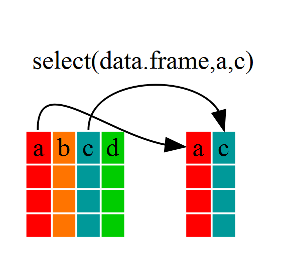
If we open up year_country_gdp we’ll see that it only contains the year, country and gdpPercap. Above we used ‘normal’ grammar, but the strengths of dplyr lie in combining several functions using pipes. Since the pipes grammar is unlike anything we’ve seen in R before, let’s repeat what we’ve done above using pipes.

R

year_country_gdp <- gapminder %>% select(year,country,gdpPercap)

To help you understand why we wrote that in that way, let’s walk through it step by step. First we summon the gapminder data frame and pass it on, using the pipe symbol %>%, to the next step, which is the select() function. In this case we don’t specify which data object we use in the select() function since in gets that from the previous pipe. Fun Fact: You may have encountered pipes before in the shell. In R, a pipe symbol is %>% while in the shell it is | but the concept is the same!

Using filter()

---

If we now wanted to move forward with the above, but only with European countries, we can combine select and filter

R

year_country_gdp_euro <- gapminder %>%
  filter(continent == "Europe") %>%
  select(year, country, gdpPercap)

Challenge 1

Write a single command (which can span multiple lines and includes pipes) that will produce a dataframe that has the African values for lifeExp, country and year, but not for other Continents. How many rows does your dataframe have and why?

Solution to Challenge 1

R

year_country_lifeExp_Africa <- gapminder %>%
                           filter(continent=="Africa") %>%
                           select(year,country,lifeExp)

As with last time, first we pass the gapminder dataframe to the filter() function, then we pass the filtered version of the gapminder data frame to the select() function. Note: The order of operations is very important in this case. If we used ‘select’ first, filter would not be able to find the variable continent since we would have removed it in the previous step.

Using group_by() and summarize()

---

Now, we were supposed to be reducing the error prone repetitiveness of what can be done with base R, but up to now we haven’t done that since we would have to repeat the above for each continent. Instead of filter(), which will only pass observations that meet your criteria (in the above: continent=="Europe"), we can use group_by(), which will essentially use every unique criteria that you could have used in filter.

R

str(gapminder)

OUTPUT

'data.frame':	1704 obs. of  6 variables:
 $ country  : chr  "Afghanistan" "Afghanistan" "Afghanistan" "Afghanistan" ...
 $ year     : int  1952 1957 1962 1967 1972 1977 1982 1987 1992 1997 ...
 $ pop      : num  8425333 9240934 10267083 11537966 13079460 ...
 $ continent: chr  "Asia" "Asia" "Asia" "Asia" ...
 $ lifeExp  : num  28.8 30.3 32 34 36.1 ...
 $ gdpPercap: num  779 821 853 836 740 ...

R

gapminder %>% group_by(continent) %>% str()

OUTPUT

gropd_df [1,704 × 6] (S3: grouped_df/tbl_df/tbl/data.frame)
 $ country  : chr [1:1704] "Afghanistan" "Afghanistan" "Afghanistan" "Afghanistan" ...
 $ year     : int [1:1704] 1952 1957 1962 1967 1972 1977 1982 1987 1992 1997 ...
 $ pop      : num [1:1704] 8425333 9240934 10267083 11537966 13079460 ...
 $ continent: chr [1:1704] "Asia" "Asia" "Asia" "Asia" ...
 $ lifeExp  : num [1:1704] 28.8 30.3 32 34 36.1 ...
 $ gdpPercap: num [1:1704] 779 821 853 836 740 ...
 - attr(*, "groups")= tibble [5 × 2] (S3: tbl_df/tbl/data.frame)
  ..$ continent: chr [1:5] "Africa" "Americas" "Asia" "Europe" ...
  ..$ .rows    : list<int> [1:5] 
  .. ..$ : int [1:624] 25 26 27 28 29 30 31 32 33 34 ...
  .. ..$ : int [1:300] 49 50 51 52 53 54 55 56 57 58 ...
  .. ..$ : int [1:396] 1 2 3 4 5 6 7 8 9 10 ...
  .. ..$ : int [1:360] 13 14 15 16 17 18 19 20 21 22 ...
  .. ..$ : int [1:24] 61 62 63 64 65 66 67 68 69 70 ...
  .. ..@ ptype: int(0) 
  ..- attr(*, ".drop")= logi TRUE

You will notice that the structure of the dataframe where we used group_by() (grouped_df) is not the same as the original gapminder (data.frame). A grouped_df can be thought of as a list where each item in the listis a data.frame which contains only the rows that correspond to the a particular value continent (at least in the example above).

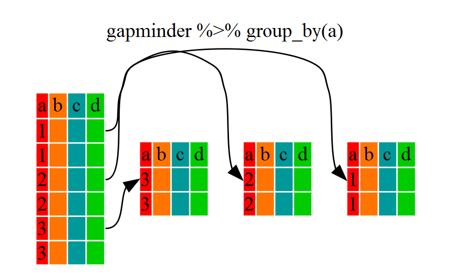
Using summarize()

---

The above was a bit on the uneventful side but group_by() is much more exciting in conjunction with summarize(). This will allow us to create new variable(s) by using functions that repeat for each of the continent-specific data frames. That is to say, using the group_by() function, we split our original dataframe into multiple pieces, then we can run functions (e.g. mean() or sd()) within summarize().

R

gdp_bycontinents <- gapminder %>%
  group_by(continent) %>%
  summarize(mean_gdpPercap = mean(gdpPercap))

gdp_bycontinents

OUTPUT

# A tibble: 5 × 2
  continent mean_gdpPercap
  <chr>              <dbl>
1 Africa             2194.
2 Americas           7136.
3 Asia               7902.
4 Europe            14469.
5 Oceania           18622.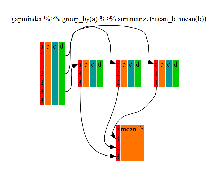

That allowed us to calculate the mean gdpPercap for each continent, but it gets even better.

Challenge 2

Calculate the average life expectancy per country. Which has the longest average life expectancy and which has the shortest average life expectancy?

Solution to Challenge 2

R

lifeExp_bycountry <- gapminder %>%
   group_by(country) %>%
   summarize(mean_lifeExp=mean(lifeExp))

lifeExp_bycountry %>%
   filter(mean_lifeExp == min(mean_lifeExp) | mean_lifeExp == max(mean_lifeExp))

OUTPUT

# A tibble: 2 × 2
  country      mean_lifeExp
  <chr>               <dbl>
1 Iceland              76.5
2 Sierra Leone         36.8

Another way to do this is to use the dplyr function arrange(), which arranges the rows in a data frame according to the order of one or more variables from the data frame. It has similar syntax to other functions from the dplyr package. You can use desc() inside arrange() to sort in descending order.

R

lifeExp_bycountry %>%
   arrange(mean_lifeExp) %>%
   head(1)

OUTPUT

# A tibble: 1 × 2
  country      mean_lifeExp
  <chr>               <dbl>
1 Sierra Leone         36.8

R

lifeExp_bycountry %>%
   arrange(desc(mean_lifeExp)) %>%
   head(1)

OUTPUT

# A tibble: 1 × 2
  country mean_lifeExp
  <chr>          <dbl>
1 Iceland         76.5

The function group_by() allows us to group by multiple variables. Let’s group by year and continent.

R

gdp_bycontinents_byyear <- gapminder %>%
  group_by(continent, year) %>%
  summarize(mean_gdpPercap = mean(gdpPercap))

OUTPUT

`summarise()` has grouped output by 'continent'. You can override using the
`.groups` argument.

That is already quite powerful, but it gets even better! You’re not limited to defining 1 new variable in summarize().

R

gdp_pop_bycontinents_byyear <- gapminder %>%
  group_by(continent,year) %>%
  summarize(mean_gdpPercap = mean(gdpPercap),
            sd_gdpPercap = sd(gdpPercap),
            mean_pop = mean(pop),
            sd_pop = sd(pop))

OUTPUT

`summarise()` has grouped output by 'continent'. You can override using the
`.groups` argument.

count() and n()

---

A very common operation is to count the number of observations for each group. The dplyr package comes with two related functions that help with this.

For instance, if we wanted to check the number of countries included in the dataset for the year 2002, we can use the count() function. It takes the name of one or more columns that contain the groups we are interested in, and we can optionally sort the results in descending order by adding sort=TRUE:

R

gapminder %>%
    filter(year == 2002) %>%
    count(continent, sort = TRUE)

OUTPUT

  continent  n
1    Africa 52
2      Asia 33
3    Europe 30
4  Americas 25
5   Oceania  2

If we need to use the number of observations in calculations, the n() function is useful. For instance, if we wanted to get the standard error of the life expectancy per continent:

R

gapminder %>%
    group_by(continent) %>%
    summarize(se_le = sd(lifeExp)/sqrt(n()))

OUTPUT

# A tibble: 5 × 2
  continent se_le
  <chr>     <dbl>
1 Africa    0.366
2 Americas  0.540
3 Asia      0.596
4 Europe    0.286
5 Oceania   0.775

You can also chain together several summary operations; in this case calculating the minimum, maximum, mean and se of each continent’s per-country life-expectancy:

R

gapminder %>%
    group_by(continent) %>%
    summarize(
      mean_le = mean(lifeExp),
      min_le = min(lifeExp),
      max_le = max(lifeExp),
      se_le = sd(lifeExp)/sqrt(n()))

OUTPUT

# A tibble: 5 × 5
  continent mean_le min_le max_le se_le
  <chr>       <dbl>  <dbl>  <dbl> <dbl>
1 Africa       48.9   23.6   76.4 0.366
2 Americas     64.7   37.6   80.7 0.540
3 Asia         60.1   28.8   82.6 0.596
4 Europe       71.9   43.6   81.8 0.286
5 Oceania      74.3   69.1   81.2 0.775

Using mutate()

---

We can also create new variables prior to (or even after) summarizing information using mutate().

R

gdp_pop_bycontinents_byyear <- gapminder %>%
  mutate(gdp_billion = gdpPercap*pop/10^9) %>%
  group_by(continent, year) %>%
  summarize(mean_gdpPercap = mean(gdpPercap),
            sd_gdpPercap = sd(gdpPercap),
            mean_pop = mean(pop),
            sd_pop = sd(pop),
            mean_gdp_billion = mean(gdp_billion),
            sd_gdp_billion = sd(gdp_billion))

OUTPUT

`summarise()` has grouped output by 'continent'. You can override using the
`.groups` argument.

Other great resources

---

• R for Data Science
• Data Wrangling Cheat sheet
• Introduction to dplyr
• Data wrangling with R and RStudio

Key Points

• Use the dplyr package to manipulate dataframes.
• Use select() to choose variables from a dataframe.
• Use filter() to choose data based on values.
• Use group_by() and summarize() to work with subsets of data.
• Use count() and n() to obtain the number of observations in columns.
• Use mutate() to create new variables.

Content from Introduction to Visualization

---

Last updated on 2024-03-12 | Edit this page

Overview

Questions

• What are the basics of creating graphics in R?

Objectives

• To be able to use ggplot2 to generate histograms and bar plots.
• To apply geometry and aesthetic layers to a ggplot plot.
• To manipulate the aesthetics of a plot using different colors and position parameters.

Plotting our data is one of the best ways to quickly explore it and the various relationships between variables. There are three main plotting systems in R, the base plotting system, the lattice package, and the ggplot2 package. Today and tomorrow we’ll be learning about the ggplot2 package, because it is the most effective for creating publication quality graphics. In this episode, we will introduce the key features of a ggplot and make a few example plots. We will expand on these concepts and see how they apply to geospatial data types when we start working with geospatial data in the R for Raster and Vector Data lesson.

ggplot2 is built on the grammar of graphics, the idea that any plot can be expressed from the same set of components: a data set, a coordinate system, and a set of geoms--the visual representation of data points. The key to understanding ggplot2 is thinking about a figure in layers. This idea may be familiar to you if you have used image editing programs like Photoshop, Illustrator, or Inkscape. In this episode we will focus on two geoms

• histograms and bar plot. In the R for Raster and Vector Data lesson we will work with a number of other geometries and learn how to customize our plots.

Let’s start off with an example plotting the distribution of life expectancy in our dataset. The first thing we do is call the ggplot function. This function lets R know that we’re creating a new plot, and any of the arguments we give the ggplot() function are the global options for the plot: they apply to all layers on the plot.

We will pass in two arguments to ggplot. First, we tell ggplot what data we want to show on our figure, in this example we use the gapminder data we read in earlier. For the second argument we pass in the aes() function, which tells ggplot how variables in the data map to aesthetic properties of the figure. Here we will tell ggplot we want to plot the “lifeExp” column of the gapminder data frame on the x-axis. We don’t need to specify a y-axis for histograms.

R

library("ggplot2")
ggplot(data = gapminder, aes(x = lifeExp)) +   
  geom_histogram()

Histogram of life expectancy by country showing bimodal distribution with modes at 45 and 75

By itself, the call to ggplot isn’t enough to draw a figure:

R

ggplot(data = gapminder, aes(x = lifeExp))

We need to tell ggplot how we want to visually represent the data, which we do by adding a geom layer. In our example, we used geom_histogram(), which tells ggplot we want to visually represent the distribution of one variable (in our case “lifeExp”):

R

ggplot(data = gapminder, aes(x = lifeExp)) +   
  geom_histogram()

OUTPUT

`stat_bin()` using `bins = 30`. Pick better value with `binwidth`.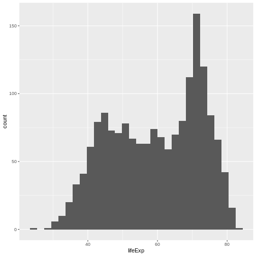

Histogram of life expectancy by country showing bimodal distribution with modes at 45 and 75

Challenge 1

Modify the example so that the figure shows the distribution of gdp per capita, rather than life expectancy:

Solution to challenge 1

R

ggplot(data = gapminder, aes(x = gdpPercap)) +   
 geom_histogram()

OUTPUT

`stat_bin()` using `bins = 30`. Pick better value with `binwidth`.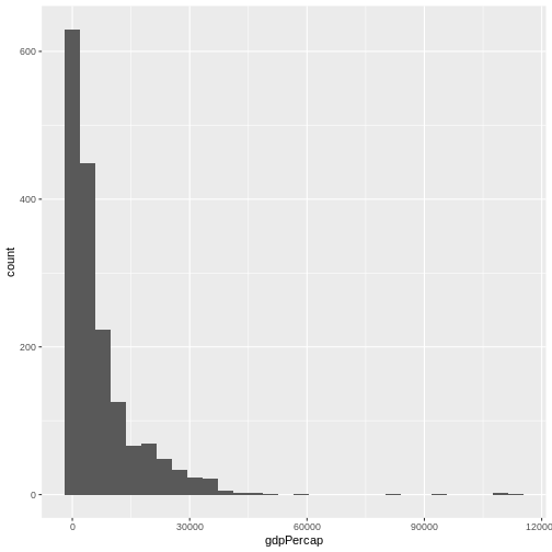

The histogram is a useful tool for visualizing the distribution of a single categorical variable. What if we want to compare the gdp per capita of the countries in our dataset? We can use a bar (or column) plot. To simplify our plot, let’s look at data only from the most recent year and only from countries in the Americas.

R

gapminder_small <- filter(gapminder, year == 2007, continent == "Americas")

This time, we will use the geom_col() function as our geometry. We will plot countries on the x-axis (listed in alphabetic order by default) and gdp per capita on the y-axis.

R

ggplot(data = gapminder_small, aes(x = country, y = gdpPercap)) + 
  geom_col()

Barplot of GDP per capita. Country names on x-axis overlap and are not readable

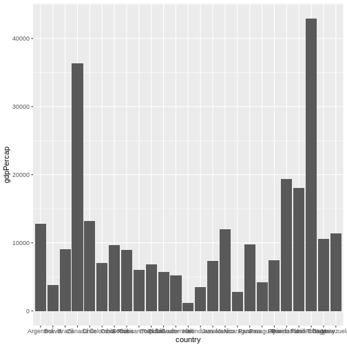
With this many bars plotted, it’s impossible to read all of the x-axis labels. A quick fix to this is the add the coord_flip() function to the end of our plot code.

R

ggplot(data = gapminder_small, aes(x = country, y = gdpPercap)) + 
  geom_col() +
  coord_flip()

Barplot showing GDP per capita. Country names on the y-axis are readable

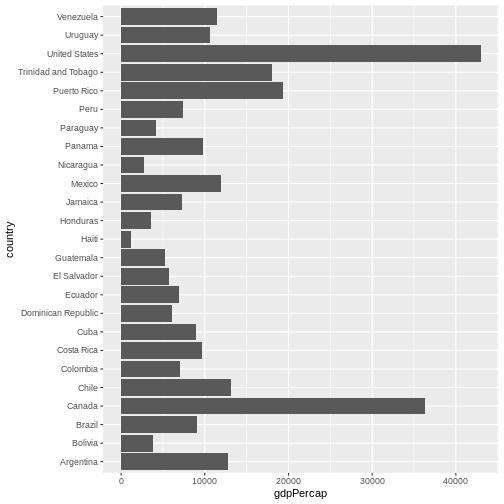
There are more sophisticated ways of modifying axis labels. We will be learning some of those methods later in this workshop.

Challenge 2

In the previous examples and challenge we’ve used the aes function to tell the geom_histogram() and geom_col() functions which columns of the data set to plot. Another aesthetic property we can modify is the color. Create a new bar (column) plot showing the gdp per capita of all countries in the Americas for the years 1952 and 2007, color coded by year.

Solution to challenge 2

First we create a new object with our filtered data:

R

gapminder_small_2 <- gapminder %>%
                        filter(continent == "Americas",
                               year %in% c(1952, 2007))

Then we plot that data using the geom_col() geom function. We color bars using the fill parameter within the aes() function. Since there are multiple bars for each country, we use the position parameter to “dodge” them so they appear side-by-side. The default behavior for postion in geom_col() is “stack”.

R

ggplot(gapminder_small_2, 
       aes(x = country, y = gdpPercap, 
       fill = as.factor(year))) +
   geom_col(position = "dodge") + 
   coord_flip()

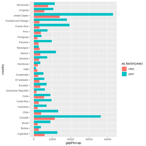
The examples given here are just the start of creating complex and beautiful graphics with R. In a later lesson we will go into much more depth, including:

• plotting geospatial specific data types
• adjusting the color scheme of our plots
• setting and formatting plot titles, subtitles, and axis labels
• creating multi-panel plots
• creating point (scatter) and line plots
• layering datasets to create multi-layered plots
• creating and customizing a plot legend
• and much more!

The examples we’ve worked through in this episode should give you the building blocks for working with the more complex graphic types and customizations we will be working with in that lesson.

Key Points

• Use ggplot2 to create plots.
• Think about graphics in layers: aesthetics, geometry, etc.

Content from Writing Data

---

Last updated on 2024-03-12 | Edit this page

Overview

Questions

• How can I save plots and data created in R?

Objectives

• To be able to write out plots and data from R.

Saving plots

---

You can save a plot from within RStudio using the ‘Export’ button in the ‘Plot’ window. This will give you the option of saving as a .pdf or as .png, .jpg or other image formats.

Sometimes you will want to save plots without creating them in the ‘Plot’ window first. Perhaps you want to make a pdf document, for example. Or perhaps you’re looping through multiple subsets of a file, plotting data from each subset, and you want to save each plot. In this case you can use flexible approach. The ggsave function saves the latest plot by default. You can control the size and resolution using the arguments to this function.

R

ggplot(data = gapminder, aes(x = gdpPercap)) +
  geom_histogram()
ggsave("Distribution-of-gdpPercap.pdf", width=12, height=4)

Open up this document and have a look.

Challenge 1

Create and save a new plot showing the side-by-side bar plot of gdp per capita in countries in the Americas in the years 1952 and 2007 that you created in the previous episode.

Solution to challenge 1

R

ggplot(data = gapminder_small_2, aes(x = country, y = gdpPercap,
                                     fill = as.factor(year))) +
  geom_col(position = "dodge") +
  coord_flip()
# Note that ggsave saves by default the latest plot.
ggsave("Distribution-of-gdpPercap.pdf", width = 12, height = 4)

To produce documents in different formats, change the file extension for jpeg, png, tiff, or bmp.

Writing data

---

At some point, you’ll also want to write out data from R.

We can use the write.csv function for this, which is very similar to read.csv from before.

Let’s create a data-cleaning script, for this analysis, we only want to focus on the gapminder data for Australia:

R

aust_subset <- filter(gapminder, country == "Australia")

write.csv(aust_subset,
  file="cleaned-data/gapminder-aus.csv"
)

Let’s open the file to make sure it contains the data we expect. Navigate to your cleaned-data directory and double-click the file name. It will open using your computer’s default for opening files with a .csv extension. To open in a specific application, right click and select the application. Using a spreadsheet program (like Excel) to open this file shows us that we do have properly formatted data including only the data points from Australia. However, there are row numbers associated with the data that are not useful to us (they refer to the row numbers from the gapminder data frame).

Let’s look at the help file to work out how to change this behaviour.

R

?write.csv

By default R will write out the row and column names when writing data to a file. To over write this behavior, we can do the following:

R

write.csv(
  aust_subset,
  file="cleaned-data/gapminder-aus.csv",
  row.names=FALSE
)

Challenge 2

Subset the gapminder data to include only data points collected since 1990. Write out the new subset to a file in the cleaned-data/ directory.

Solution to challenge 2

R

gapminder_after_1990 <- filter(gapminder, year > 1990)

write.csv(gapminder_after_1990,
  file = "cleaned-data/gapminder-after-1990.csv",
  row.names = FALSE)

Key Points

• Save plots using ggsave().
• Use write.csv to save tabular data.