Introduction to R and RStudio
Last updated on 2024-10-16 | Edit this page
Overview
Questions
- How to find your way around RStudio?
- How to interact with R?
- How to install packages?
Objectives
- Describe the purpose and use of each pane in the RStudio IDE
- Locate buttons and options in the RStudio IDE
- Define a variable
- Assign data to a variable
- Use mathematical and comparison operators
- Call functions
- Manage packages
Motivation
Science is a multi-step process: once you’ve designed an experiment and collected data, the real fun begins! This lesson will teach you how to start this process using R and RStudio. We will begin with raw data, perform exploratory analyses, and learn how to plot results graphically. This example starts with a dataset from gapminder.org containing population information for many countries through time. Can you read the data into R? Can you plot the population for Senegal? Can you calculate the average income for countries on the continent of Asia? By the end of these lessons you will be able to do things like plot the populations for all of these countries in under a minute!
Before Starting The Workshop
Please ensure you have the latest version of R and RStudio installed on your machine. This is important, as some packages used in the workshop may not install correctly (or at all) if R is not up to date.
Introduction to RStudio
Throughout this lesson, we’re going to teach you some of the fundamentals of the R language as well as some best practices for organizing code for scientific projects that will make your life easier.
We’ll be using RStudio: a free, open source R integrated development environment (IDE). It provides a built in editor, works on all platforms (including on servers) and provides many advantages such as integration with version control and project management.
Basic layout
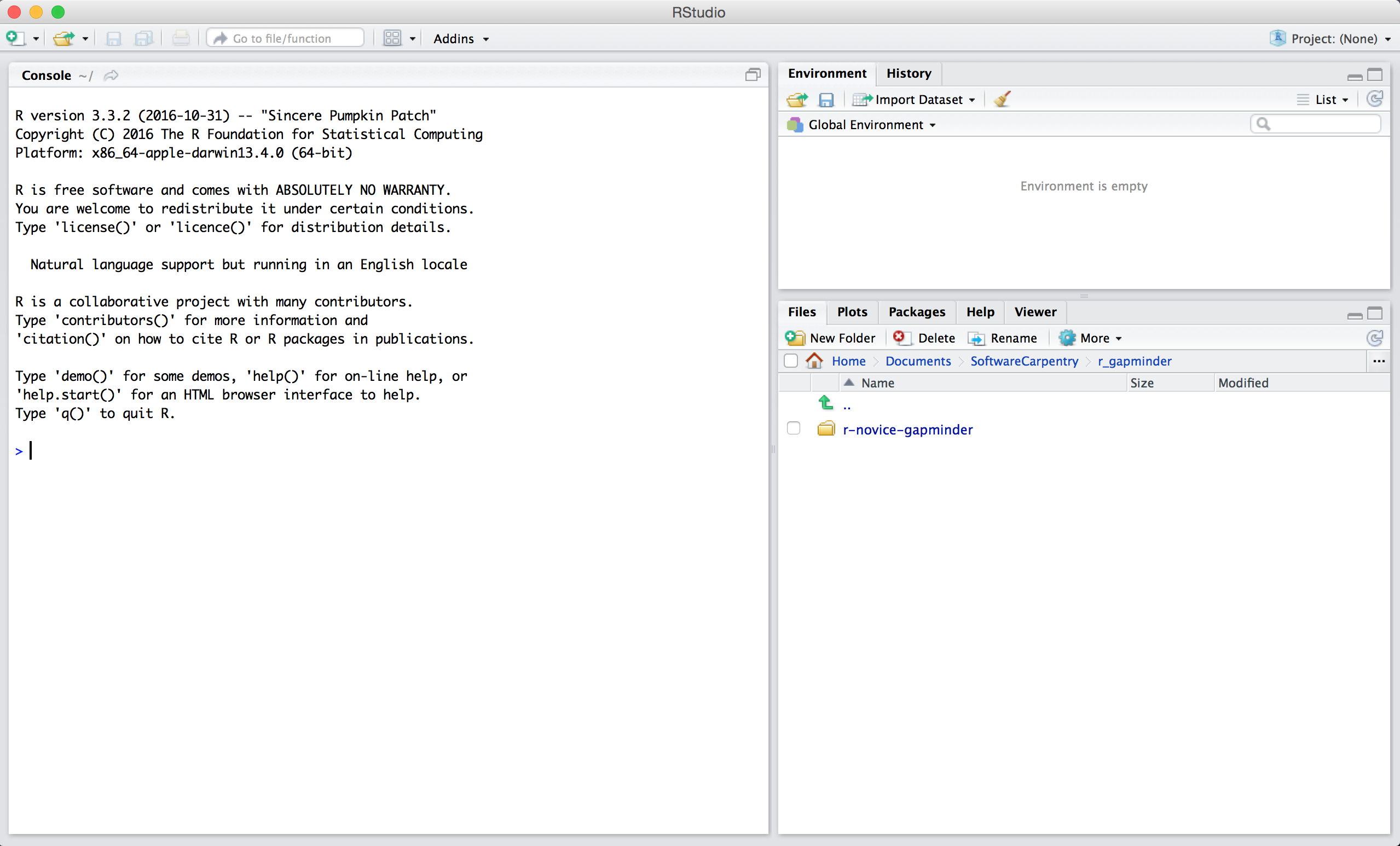
When you first open RStudio, you will be greeted by three panels:
- The interactive R console (entire left)
- Environment/History (tabbed in upper right)
- Files/Plots/Packages/Help/Viewer (tabbed in lower right)
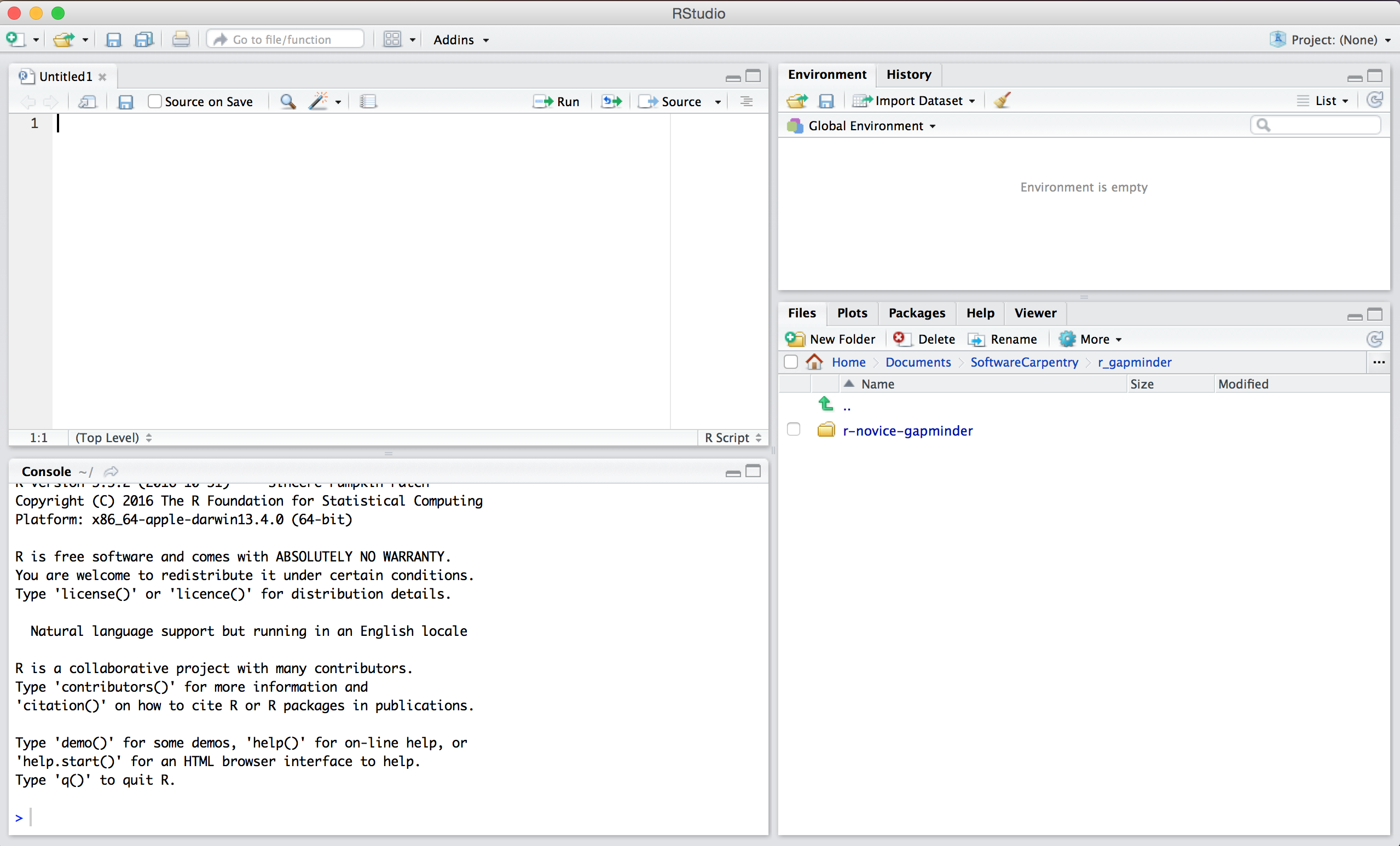
Once you open files, such as R scripts, an editor panel will also open in the top left.
Workflow within RStudio
There are two main ways one can work within RStudio.
- Test and play within the interactive R console then copy code into a .R file to run later.
- This works well when doing small tests and initially starting off.
- It quickly becomes laborious
- Start writing in an .R file and use RStudio’s shortcut keys for the Run command to push the current line, selected lines or modified lines to the interactive R console.
- This is a great way to start; all your code is saved for later
- You will be able to run the file you create from within RStudio or
using R’s
source()function.
Tip: Running segments of your code
RStudio offers you great flexibility in running code from within the editor window. There are buttons, menu choices, and keyboard shortcuts. To run the current line, you can
- click on the
Runbutton above the editor panel, or - select “Run Lines” from the “Code” menu, or
- hit Ctrl+Enter in Windows,
Ctrl+Return in Linux, or
⌘+Return on OS X. (This shortcut can also be seen
by hovering the mouse over the button). To run a block of code, select
it and then
Run. If you have modified a line of code within a block of code you have just run, there is no need to reselect the section andRun, you can use the next button along,Re-run the previous region. This will run the previous code block including the modifications you have made.
Introduction to R
Much of your time in R will be spent in the R interactive console.
This is where you will run all of your code, and can be a useful
environment to try out ideas before adding them to an R script file.
This console in RStudio is the same as the one you would get if you
typed in R in your command-line environment.
The first thing you will see in the R interactive session is a bunch of information, followed by a “>” and a blinking cursor. When you are running a section of your code, this is the location where R will first read your code, attempt to execute them, and then returns a result.
Using R as a calculator
The simplest thing you could do with R is do arithmetic:
R
1 + 100
OUTPUT
[1] 101And R will print out the answer, with a preceding “[1]”.
Don’t worry about this for now, we’ll explain that later. For now think
of it as indicating output.
Like bash, if you type in an incomplete command, R will wait for you to complete it:
OUTPUT
+Any time you hit return and the R session shows a “+”
instead of a “>”, it means it’s waiting for you to
complete the command. If you want to cancel a command you can simply hit
“Esc” and RStudio will give you back the “>”
prompt.
Tip: Cancelling commands
If you’re using R from the command line instead of from within RStudio, you need to use Ctrl+C instead of Esc to cancel the command. This applies to Mac users as well!
Cancelling a command isn’t only useful for killing incomplete commands: you can also use it to tell R to stop running code (for example if it’s taking much longer than you expect), or to get rid of the code you’re currently writing.
When using R as a calculator, the order of operations is the same as you would have learned back in school.
From highest to lowest precedence:
- Parentheses:
(,) - Exponents:
^or** - Divide:
/ - Multiply:
* - Add:
+ - Subtract:
-
R
3 + 5 * 2
OUTPUT
[1] 13Use parentheses to group operations in order to force the order of evaluation if it differs from the default, or to make clear what you intend.
R
(3 + 5) * 2
OUTPUT
[1] 16This can get unwieldy when not needed, but clarifies your intentions. Remember that others may later read your code.
R
(3 + (5 * (2 ^ 2))) # hard to read
3 + 5 * 2 ^ 2       # clear, if you remember the rules
3 + 5 * (2 ^ 2)     # if you forget some rules, this might help
The text after each line of code is called a “comment”. Anything that
follows after the hash (or octothorpe) symbol # is ignored
by R when it executes code.
Really small or large numbers get a scientific notation:
R
2/10000
OUTPUT
[1] 2e-04Which is shorthand for “multiplied by 10^XX”. So
2e-4 is shorthand for 2 * 10^(-4).
You can write numbers in scientific notation too:
R
5e3 # Note the lack of minus here
OUTPUT
[1] 5000Don’t worry about trying to remember every function in R. You can look them up using a search engine, or if you can remember the start of the function’s name, use the tab completion in RStudio.
This is one advantage that RStudio has over R on its own, it has auto-completion abilities that allow you to more easily look up functions, their arguments, and the values that they take.
Typing a ? before the name of a command will open the
help page for that command. As well as providing a detailed description
of the command and how it works, scrolling to the bottom of the help
page will usually show a collection of code examples which illustrate
command usage. We’ll go through an example later.
Comparing things
We can also do comparison in R:
R
1 == 1 # equality (note two equals signs, read as "is equal to")
OUTPUT
[1] TRUER
1 != 2 # inequality (read as "is not equal to")
OUTPUT
[1] TRUER
1 < 2 # less than
OUTPUT
[1] TRUER
1 <= 1 # less than or equal to
OUTPUT
[1] TRUER
1 > 0 # greater than
OUTPUT
[1] TRUER
1 >= -9 # greater than or equal to
OUTPUT
[1] TRUETip: Comparing Numbers
A word of warning about comparing numbers: you should never use
== to compare two numbers unless they are integers (a data
type which can specifically represent only whole numbers).
Computers may only represent decimal numbers with a certain degree of precision, so two numbers which look the same when printed out by R, may actually have different underlying representations and therefore be different by a small margin of error (called Machine numeric tolerance).
Instead you should use the all.equal function.
Further reading: http://floating-point-gui.de/
Variables and assignment
We can store values in variables using the assignment operator
<-, like this:
R
x <- 1/40
Notice that assignment does not print a value. Instead, we stored it
for later in something called a variable.
x now contains the value
0.025:
R
x
OUTPUT
[1] 0.025More precisely, the stored value is a decimal approximation of this fraction called a floating point number.
Look for the Environment tab in one of the panes of
RStudio, and you will see that x and its value have
appeared. Our variable x can be used in place of a number
in any calculation that expects a number:
R
log(x)
OUTPUT
[1] -3.688879Notice also that variables can be reassigned:
R
x <- 100
x used to contain the value 0.025 and and now it has the
value 100.
Assignment values can contain the variable being assigned to:
R
x <- x + 1 #notice how RStudio updates its description of x on the top right tab
y <- x * 2
The right hand side of the assignment can be any valid R expression. The right hand side is fully evaluated before the assignment occurs.
Challenge 1
What will be the value of each variable after each statement in the following program?
R
mass <- 47.5
age <- 122
mass <- mass * 2.3
age <- age - 20
R
mass <- 47.5
This will give a value of 47.5 for the variable mass
R
age <- 122
This will give a value of 122 for the variable age
R
mass <- mass * 2.3
This will multiply the existing value of 47.5 by 2.3 to give a new value of 109.25 to the variable mass.
R
age <- age - 20
This will subtract 20 from the existing value of 122 to give a new value of 102 to the variable age.
Challenge 2
Run the code from the previous challenge, and write a command to compare mass to age. Is mass larger than age?
One way of answering this question in R is to use the
> to set up the following:
R
mass > age
OUTPUT
[1] TRUEThis should yield a boolean value of TRUE since 109.25 is greater than 102.
Variable names can contain letters, numbers, underscores and periods. They cannot start with a number nor contain spaces at all. Different people use different conventions for long variable names, these include
- periods.between.words
- underscores_between_words
- camelCaseToSeparateWords
What you use is up to you, but be consistent.
It is also possible to use the = operator for
assignment:
R
x = 1/40
But this is much less common among R users. The most important thing
is to be consistent with the operator you use. There
are occasionally places where it is less confusing to use
<- than =, and it is the most common symbol
used in the community. So the recommendation is to use
<-.
The following can be used as R variables:
R
min_height
max.height
MaxLength
celsius2kelvin
The following creates a hidden variable:
R
.mass
We won’t be discussing hidden variables in this lesson. We recommend not using a period at the beginning of variable names unless you intend your variables to be hidden.
The following will not be able to be used to create a variable
Installing Packages
We can use R as a calculator to do mathematical operations (e.g., addition, subtraction, multiplication, division), as we did above. However, we can also use R to carry out more complicated analyses, make visualizations, and much more. In later episodes, we’ll use R to do some data wrangling, plotting, and saving of reformatted data.
R coders around the world have developed collections of R code to accomplish themed tasks (e.g., data wrangling). These collections of R code are known as R packages. It is also important to note that R packages refer to code that is not automatically downloaded when we install R on our computer. Therefore, we’ll have to install each R package that we want to use (more on this below).
We will practice using the dplyr package to wrangle our
datasets in episode 6 and will also practice using the
ggplot2 package to plot our data in episode 7. To give an
example, the dplyr package includes code for a function
called filter(). A function is something that
takes input(s) does some internal operations and produces output(s). For
the filter() function, the inputs are a dataset and a
logical statement (i.e., when data value is greater than or equal to
100) and the output is data within the dataset that has a value greater
than or equal to 100.
There are two main ways to install packages in R:
If you are using RStudio, we can go to
Tools>Install Packages...and then search for the name of the R package we need and clickInstall.We can use the
install.packages( )function. We can do this to install thedplyrR package.
R
install.packages("dplyr")
OUTPUT
The following package(s) will be installed:
- dplyr [1.1.4]
These packages will be installed into "~/work/r-intro-geospatial/r-intro-geospatial/renv/profiles/lesson-requirements/renv/library/linux-ubuntu-jammy/R-4.4/x86_64-pc-linux-gnu".

# Installing packages --------------------------------------------------------
- Installing dplyr ...                          OK [linked from cache]
Successfully installed 1 package in 7.8 milliseconds.
It’s important to note that we only need to install the R package on our computer once. Well, if we install a new version of R on the same computer, then we will likely need to also re-install the R packages too.
Challenge 4
What code would we use to install the ggplot2
package?
We would use the following R code to install the ggplot2
package:
R
install.packages("ggplot2")
Now that we’ve installed the R package, we’re ready to use it! To use the R package, we need to “load” it into our R session. We can think of “loading” an R packages as telling R that we’re ready to use the package we just installed. It’s important to note that while we only have to install the package once, we’ll have to load the package each time we open R (or RStudio).
To load an R package, we use the library( ) function. We
can load the dplyr package like this:
R
library(dplyr)
OUTPUT
Attaching package: 'dplyr'OUTPUT
The following objects are masked from 'package:stats':

    filter, lag
OUTPUT
The following objects are masked from 'package:base':

    intersect, setdiff, setequal, union
Challenge 5
Which of the following could we use to load the ggplot2
package? (Select all that apply.)
- install.packages(“ggplot2”)
- library(“ggplot2”)
- library(ggplot2)
- library(ggplo2)
The correct answers are b and c. Answer a will install, not load, the ggplot2 package. Answer b will correctly load the ggplot2 package. Note there are no quotation marks. Answer c will correctly load the ggplot2 package. Note there are quotation marks. Answer d will produce an error because ggplot2 is misspelled.
Note: It is more common for coders to not use quotation marks when loading an R package (i.e., answer c).
R
library(ggplot2)
Key Points
- Use RStudio to write and run R programs.
- R has the usual arithmetic operators.
- Use
<-to assign values to variables. - Use
install.packages()to install packages (libraries).