Content from Introduction to Raster Data
Last updated on 2023-08-15 | Edit this page
Overview
Questions
- What format should I use to represent my data?
- What are the main data types used for representing geospatial data?
- What are the main attributes of raster data?
Objectives
- Describe the difference between raster and vector data.
- Describe the strengths and weaknesses of storing data in raster format.
- Distinguish between continuous and categorical raster data and identify types of datasets that would be stored in each format.
This episode introduces the two primary types of geospatial data: rasters and vectors. After briefly introducing these data types, this episode focuses on raster data, describing some major features and types of raster data.
Data Structures: Raster and Vector
The two primary types of geospatial data are raster and vector data. Raster data is stored as a grid of values which are rendered on a map as pixels. Each pixel value represents an area on the Earth’s surface. Vector data structures represent specific features on the Earth’s surface, and assign attributes to those features. Vector data structures will be discussed in more detail in the next episode.
The R for Raster and Vector Data lesson will focus on how to work with both raster and vector data sets, therefore it is essential that we understand the basic structures of these types of data and the types of data that they can be used to represent.
About Raster Data
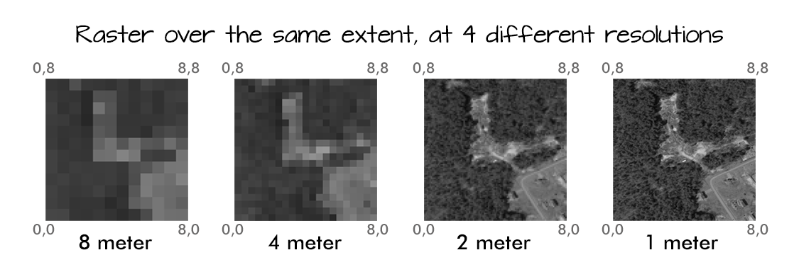
Raster data is any pixelated (or gridded) data where each pixel is associated with a specific geographical location. The value of a pixel can be continuous (e.g. elevation) or categorical (e.g. land use). If this sounds familiar, it is because this data structure is very common: it’s how we represent any digital image. A geospatial raster is only different from a digital photo in that it is accompanied by spatial information that connects the data to a particular location. This includes the raster’s extent and cell size, the number of rows and columns, and its coordinate reference system (or CRS).
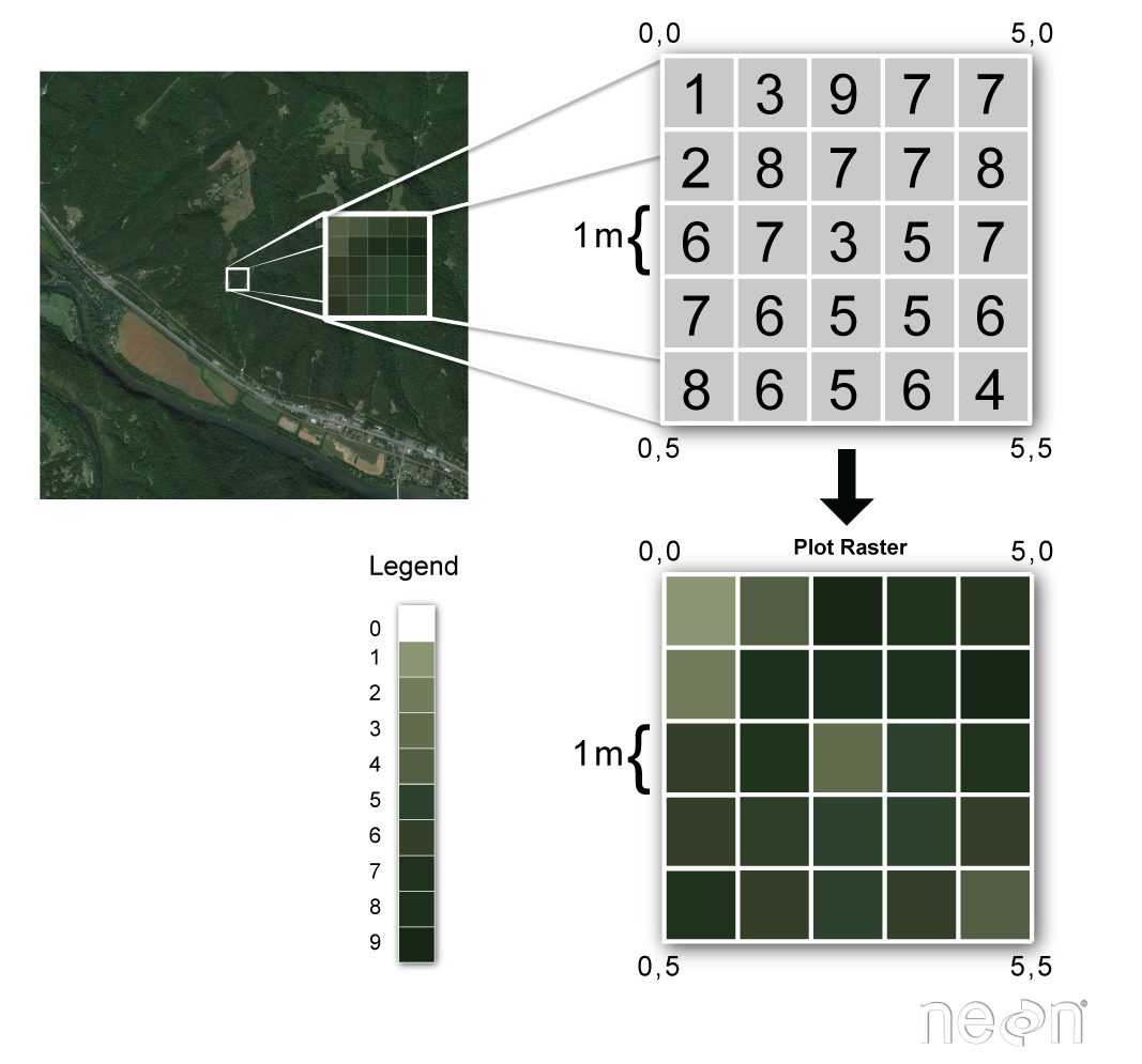
Source: National Ecological Observatory Network (NEON) {: .text-center}
Some examples of continuous rasters include:
- Precipitation maps.
- Maps of tree height derived from LiDAR data.
- Elevation values for a region.
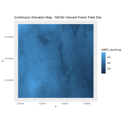
A map of elevation for Harvard Forest derived from the NEON AOP LiDAR sensor is below. Elevation is represented as continuous numeric variable in this map. The legend shows the continuous range of values in the data from around 300 to 420 meters.
Some rasters contain categorical data where each pixel represents a discrete class such as a landcover type (e.g., “forest” or “grassland”) rather than a continuous value such as elevation or temperature. Some examples of classified maps include:
- Landcover / land-use maps.
- Tree height maps classified as short, medium, and tall trees.
- Elevation maps classified as low, medium, and high elevation.
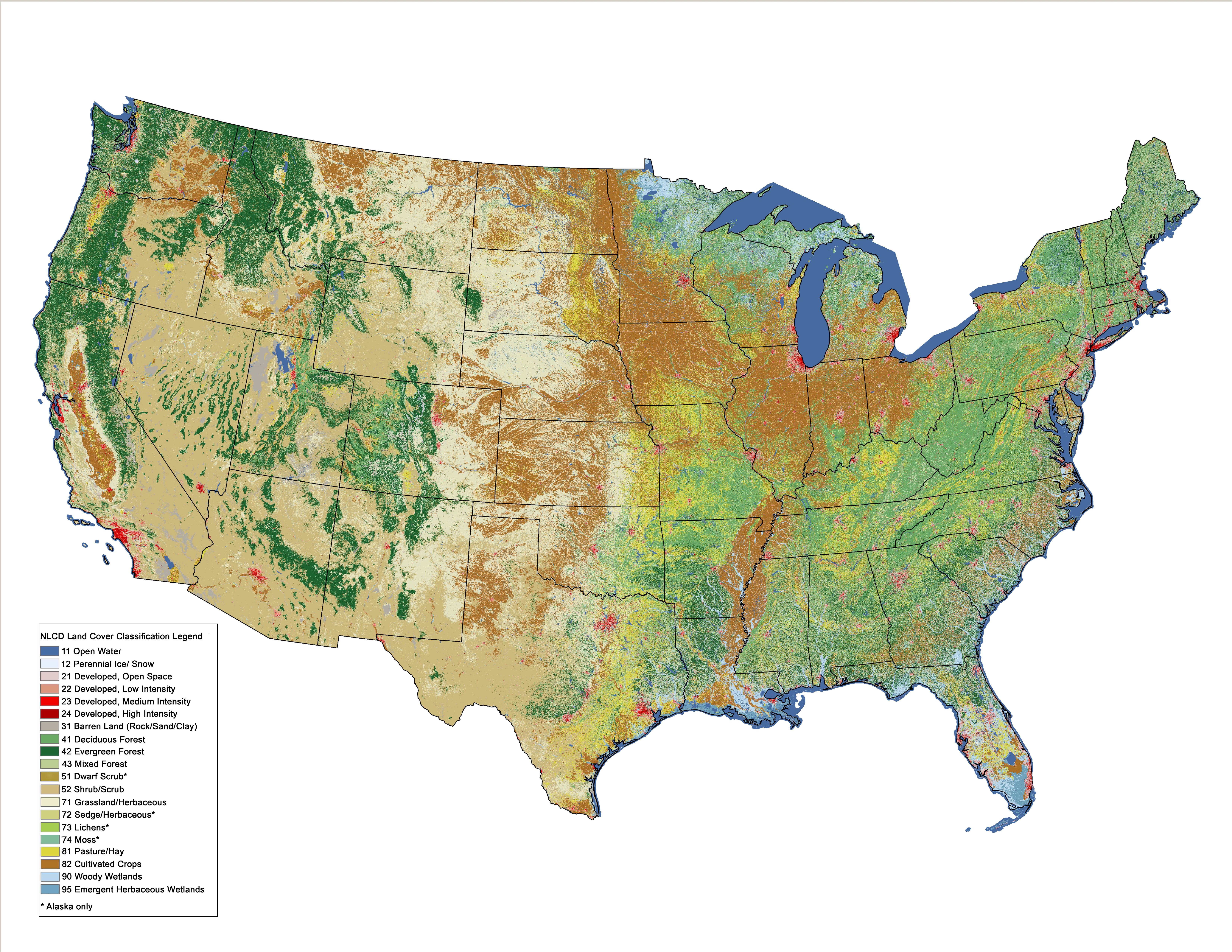
The map above shows the contiguous United States with landcover as categorical data. Each color is a different landcover category. (Source: Homer, C.G., et al., 2015, Completion of the 2011 National Land Cover Database for the conterminous United States-Representing a decade of land cover change information. Photogrammetric Engineering and Remote Sensing, v. 81, no. 5, p. 345-354)
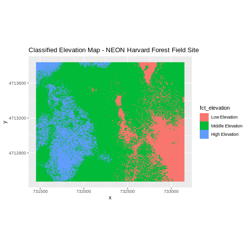
The map above shows elevation data for the NEON Harvard Forest field site. We will be working with data from this site later in the workshop. In this map, the elevation data (a continuous variable) has been divided up into categories to yield a categorical raster.
Raster data has some important advantages:
- representation of continuous surfaces
- potentially very high levels of detail
- data is ‘unweighted’ across its extent - the geometry doesn’t implicitly highlight features
- cell-by-cell calculations can be very fast and efficient
The downsides of raster data are:
- very large file sizes as cell size gets smaller
- currently popular formats don’t embed metadata well (more on this later!)
- can be difficult to represent complex information
Important Attributes of Raster Data
Extent
The spatial extent is the geographic area that the raster data covers. The spatial extent of an R spatial object represents the geographic edge or location that is the furthest north, south, east and west. In other words, extent represents the overall geographic coverage of the spatial object.
(Image Source: National Ecological Observatory Network (NEON)) {: .text-center}
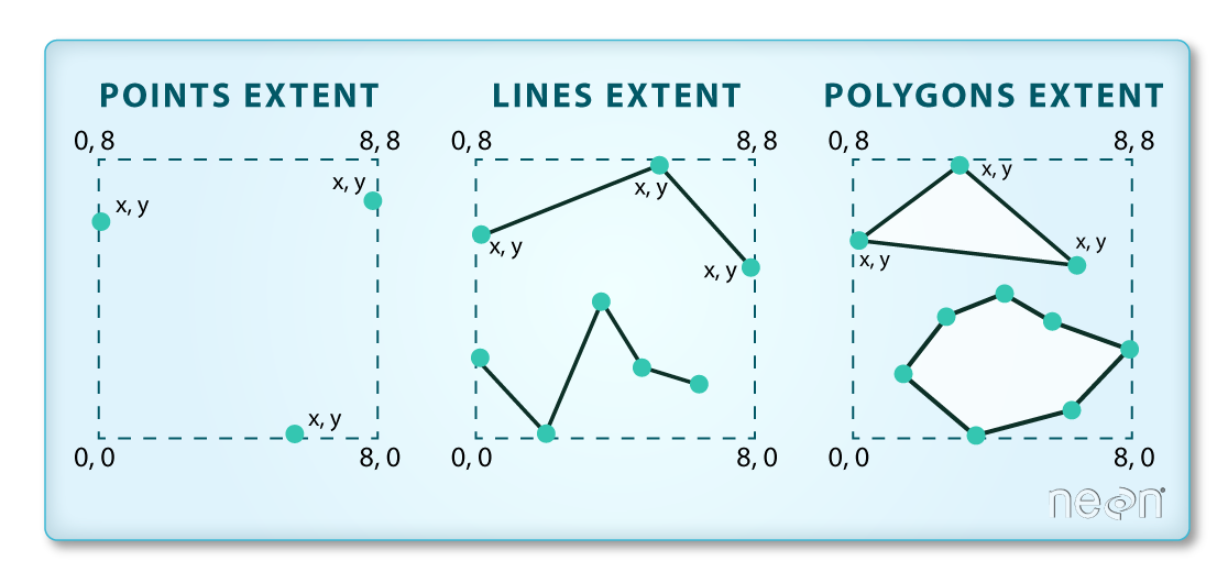
The lines and polygon objects have the same extent. The extent for the points object is smaller in the vertical direction than the other two because there are no points on the line at y = 8.
Raster Data Format for this Workshop
Raster data can come in many different formats. For this workshop, we
will use the GeoTIFF format which has the extension .tif. A
.tif file stores metadata or attributes about the file as
embedded tif tags. For instance, your camera might store a
tag that describes the make and model of the camera or the date the
photo was taken when it saves a .tif. A GeoTIFF is a
standard .tif image format with additional spatial
(georeferencing) information embedded in the file as tags. These tags
should include the following raster metadata:
- Extent
- Resolution
- Coordinate Reference System (CRS) - we will introduce this concept in a later episode
- Values that represent missing data (
NoDataValue) - we will introduce this concept in a later lesson.
We will discuss these attributes in more detail in a later lesson. In that lesson, we will also learn how to use R to extract raster attributes from a GeoTIFF file.
Multi-band Raster Data
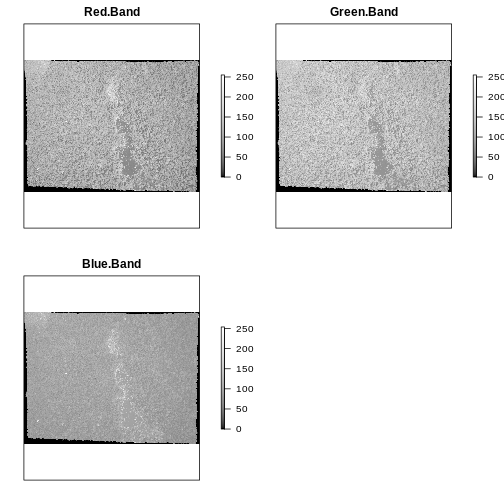
A raster can contain one or more bands. One type of multi-band raster dataset that is familiar to many of us is a color image. A basic color image consists of three bands: red, green, and blue. Each band represents light reflected from the red, green or blue portions of the electromagnetic spectrum. The pixel brightness for each band, when composited creates the colors that we see in an image.

(Source: National Ecological Observatory Network (NEON).) {: .text-center}
We can plot each band of a multi-band image individually.
Or we can composite all three bands together to make a color image.
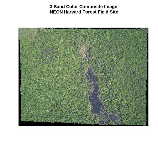
In a multi-band dataset, the rasters will always have the same extent, resolution, and CRS.
Other Types of Multi-band Raster Data
Multi-band raster data might also contain:
- Time series: the same variable, over the same area, over time. We will be working with time series data in the Raster Time Series Data in R episode.
- Multi or hyperspectral imagery: image rasters that have 4 or more (multi-spectral) or more than 10-15 (hyperspectral) bands. We won’t be working with this type of data in this workshop, but you can check out the NEON Data Skills Imaging Spectroscopy HDF5 in R tutorial if you’re interested in working with hyperspectral data cubes.
Content from Introduction to Vector Data
Last updated on 2023-08-15 | Edit this page
Overview
Questions
- What are the main attributes of vector data?
Objectives
- Describe the strengths and weaknesses of storing data in vector format.
- Describe the three types of vectors and identify types of data that would be stored in each.
About Vector Data
Vector data structures represent specific features on the Earth’s surface, and assign attributes to those features. Vectors are composed of discrete geometric locations (x, y values) known as vertices that define the shape of the spatial object. The organization of the vertices determines the type of vector that we are working with: point, line or polygon.
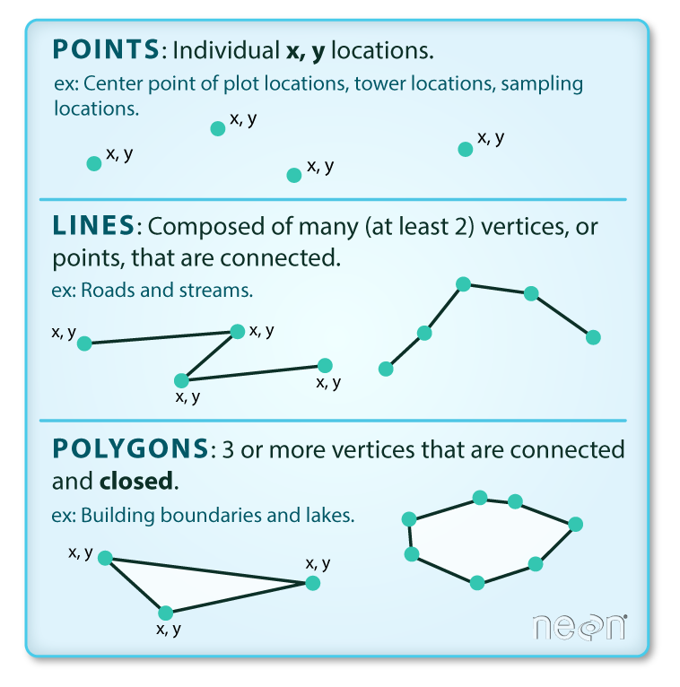
Image Source: National Ecological Observatory Network (NEON) {: .text-center}
Points: Each point is defined by a single x, y coordinate. There can be many points in a vector point file. Examples of point data include: sampling locations, the location of individual trees, or the location of survey plots.
Lines: Lines are composed of many (at least 2) points that are connected. For instance, a road or a stream may be represented by a line. This line is composed of a series of segments, each “bend” in the road or stream represents a vertex that has defined x, y location.
Polygons: A polygon consists of 3 or more vertices that are connected and closed. The outlines of survey plot boundaries, lakes, oceans, and states or countries are often represented by polygons.
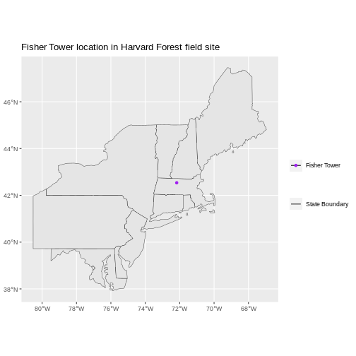
State boundaries are polygons. The Fisher Tower location is a point. There are no line features shown.
Vector data has some important advantages:
- The geometry itself contains information about what the dataset creator thought was important
- The geometry structures hold information in themselves - why choose point over polygon, for instance?
- Each geometry feature can carry multiple attributes instead of just one, e.g. a database of cities can have attributes for name, country, population, etc
- Data storage can be very efficient compared to rasters
The downsides of vector data include:
- potential loss of detail compared to raster
- potential bias in datasets - what didn’t get recorded?
- Calculations involving multiple vector layers need to do math on the geometry as well as the attributes, so can be slow compared to raster math.
Vector datasets are in use in many industries besides geospatial fields. For instance, computer graphics are largely vector-based, although the data structures in use tend to join points using arcs and complex curves rather than straight lines. Computer-aided design (CAD) is also vector- based. The difference is that geospatial datasets are accompanied by information tying their features to real-world locations.
Vector Data Format for this Workshop
Like raster data, vector data can also come in many different
formats. For this workshop, we will use the Shapefile format which has
the extension .shp. A .shp file stores the
geographic coordinates of each vertice in the vector, as well as
metadata including:
- Extent - the spatial extent of the shapefile (i.e. geographic area that the shapefile covers). The spatial extent for a shapefile represents the combined extent for all spatial objects in the shapefile.
- Object type - whether the shapefile includes points, lines, or polygons.
- Coordinate reference system (CRS)
- Other attributes - for example, a line shapefile that contains the locations of streams, might contain the name of each stream.
Because the structure of points, lines, and polygons are different, each individual shapefile can only contain one vector type (all points, all lines or all polygons). You will not find a mixture of point, line and polygon objects in a single shapefile.
More Resources
More about shapefiles can be found on Wikipedia
Why not both?
Very few formats can contain both raster and vector data - in fact, most are even more restrictive than that. Vector datasets are usually locked to one geometry type, e.g. points only. Raster datasets can usually only encode one data type, for example you can’t have a multiband GeoTIFF where one layer is integer data and another is floating-point. There are sound reasons for this - format standards are easier to define and maintain, and so is metadata. The effects of particular data manipulations are more predictable if you are confident that all of your input data has the same characteristics.
Content from Coordinate Reference Systems
Last updated on 2023-08-15 | Edit this page
Overview
Questions
- What is a coordinate reference system and how do I interpret one?
Objectives
- Name some common schemes for describing coordinate reference systems.
- Interpret a PROJ4 coordinate reference system description.
Coordinate Reference Systems
A data structure cannot be considered geospatial unless it is accompanied by coordinate reference system (CRS) information, in a format that geospatial applications can use to display and manipulate the data correctly. CRS information connects data to the Earth’s surface using a mathematical model.
The CRS associated with a dataset tells your mapping software (for example R) where the raster is located in geographic space. It also tells the mapping software what method should be used to flatten or project the raster in geographic space.
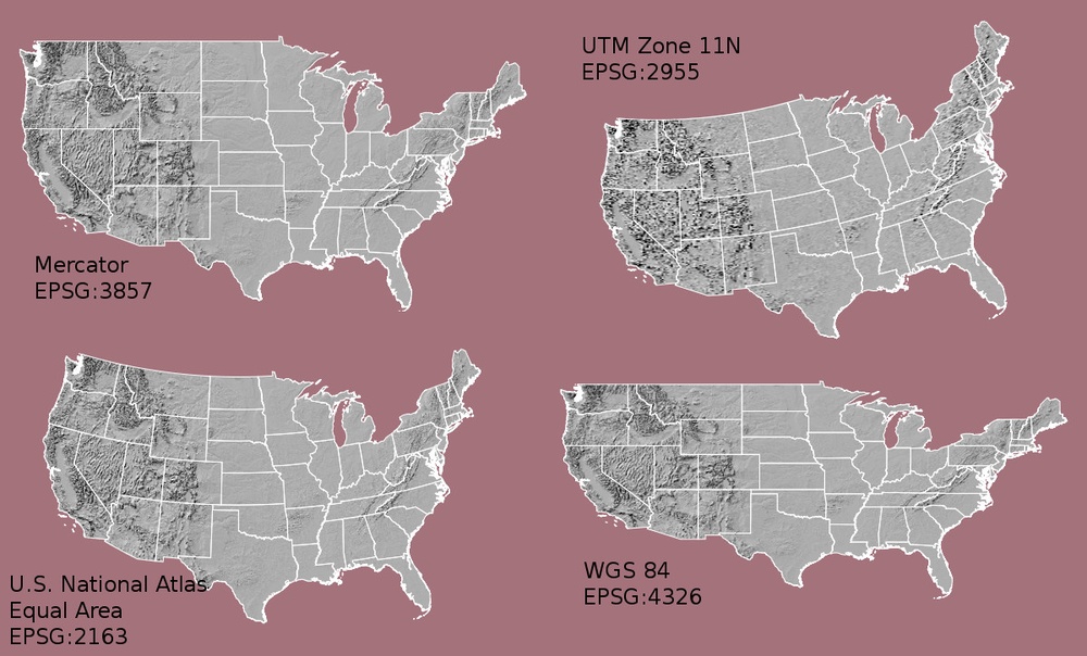
The above image shows maps of the United States in different projections. Notice the differences in shape associated with each projection. These differences are a direct result of the calculations used to flatten the data onto a 2-dimensional map. (Source: opennews.org) {: .text-center}
There are lots of great resources that describe coordinate reference systems and projections in greater detail. For the purposes of this workshop, what is important to understand is that data from the same location but saved in different projections will not line up in any GIS or other program. Thus, it’s important when working with spatial data to identify the coordinate reference system applied to the data and retain it throughout data processing and analysis.
Components of a CRS
CRS information has three components:
Datum: A model of the shape of the earth. It has angular units (i.e. degrees) and defines the starting point (i.e. where is (0,0)?) so the angles reference a meaningful spot on the earth. Common global datums are WGS84 and NAD83. Datums can also be local - fit to a particular area of the globe, but ill-fitting outside the area of intended use. In this workshop, we will use the WGS84 datum.
Projection: A mathematical transformation of the angular measurements on a round earth to a flat surface (i.e. paper or a computer screen). The units associated with a given projection are usually linear (feet, meters, etc.). In this workshop, we will see data in two different projections.
Additional Parameters: Additional parameters are often necessary to create the full coordinate reference system. One common additional parameter is a definition of the center of the map. The number of required additional parameters depends on what is needed by each specific projection.
Orange Peel Analogy
A common analogy employed to teach projections is the orange peel analogy. If you imagine that the earth is an orange, how you peel it and then flatten the peel is similar to how projections get made.
- A datum is the choice of fruit to use. Is the earth an orange, a lemon, a lime, a grapefruit?

Image source {: .text-center}
A projection is how you peel your orange and then flatten the peel.
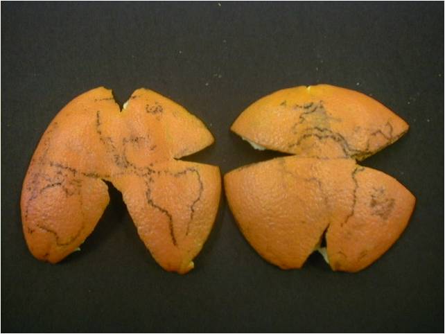
Image source {: .text-center}
- An additional parameter could include a definition of the location of the stem of the fruit. What other parameters could be included in this analogy?
Which projection should I use?
To decide if a projection is right for your data, answer these questions:
- What is the area of minimal distortion?
- What aspect of the data does it preserve?
University of Colorado’s Map Projections and the Department of Geo-Information Processing has a good discussion of these aspects of projections. Online tools like Projection Wizard can also help you discover projections that might be a good fit for your data.
Describing Coordinate Reference Systems
There are several common systems in use for storing and transmitting CRS information, as well as translating among different CRSs. These systems generally comply with ISO 19111. Common systems for describing CRSs include EPSG, PROJ, and OGC WKT. Most of the data we will be working with in this workshop use the PROJ system.
PROJ is an open-source library for storing, representing and transforming CRS information. PROJ.5 has been recently released, but PROJ.4 was in use for 25 years so you will still mostly see PROJ referred to as PROJ.4. PROJ represents CRS information as a text string of key-value pairs, which makes it easy to customise (and with a little practice, easy to read and interpret).
A PROJ4 string includes the following information:
- proj=: the projection of the data
- zone=: the zone of the data (this is specific to the UTM projection)
- datum=: the datum use
- units=: the units for the coordinates of the data
- ellps=: the ellipsoid (how the earth’s roundness is calculated) for the data
Note that the zone is unique to the UTM projection. Not all CRSs will have a zone.

Image source: Chrismurf at English Wikipedia, via Wikimedia Commons (CC-BY). {: .text-center}
Reading a PROJ4 String
Here is a PROJ4 string for one of the datasets we will use in this workshop:
+proj=utm +zone=18 +datum=WGS84 +units=m +no_defs +ellps=WGS84 +towgs84=0,0,0
- What projection, zone, datum, and ellipsoid are used for this data?
- What are the units of the data?
- Using the map above, what part of the United States was this data collected from?
- Projection is UTM, zone 18, datum is WGS84, ellipsoid is WGS84.
- The data is in meters.
- The data comes from the eastern US seaboard.
Other Common Systems
The EPSG system is a database of CRS information maintained by the International Association of Oil and Gas Producers. The dataset contains both CRS definitions and information on how to safely convert data from one CRS to another. Using EPSG is easy as every CRS has a integer identifier, e.g. WGS84 is EPSG:4326. The downside is that you can only use the CRSs EPSG defines and cannot customise them. Detailed information on the structure of the EPSG dataset is available on their website.
The OGC WKT standard is used by a number of important geospatial apps and software libraries. WKT is a nested list of geodetic parameters. The structure of the information is defined on their website. WKT is valuable in that the CRS information is more transparent than in EPSG, but can be more difficult to read and compare than PROJ. Additionally, the WKT standard is implemented inconsistently across various software platforms, and the spec itself has some known issues).
Format interoperability
Many existing file formats were invented by GIS software developers, often in a closed-source environment. This led to the large number of formats on offer today, and considerable problems transferring data between software environments. The Geospatial Data Abstraction Library (GDAL) is an open-source answer to this issue.
GDAL is a set of software tools that translate between almost any geospatial format in common use today (and some not so common ones). GDAL also contains tools for editing and manipulating both raster and vector files, including reprojecting data to different CRSs. GDAL can be used as a standalone command-line tool, or built in to other GIS software. Several open-source GIS programs use GDAL for all file import/export operations. We will be working with GDAL later in this workshop.
Metadata
Spatial data is useless without metadata. Essential metadata includes the CRS information, but proper spatial metadata encompasses more than that. History and provenance of a dataset (how it was made), who is in charge of maintaining it, and appropriate (and inappropriate!) use cases should also be documented in metadata. This information should accompany a spatial dataset wherever it goes. In practice this can be difficult, as many spatial data formats don’t have a built-in place to hold this kind of information. Metadata often has to be stored in a companion file, and generated and maintained manually.
More Resources on CRS
- spatialreference.org - A comprehensive online library of CRS information.
- QGIS Documentation - CRS Overview.
- Choosing the Right Map Projection.
- NCEAS Overview of CRS in R.
- Video highlighting how map projections can make continents seems proportionally larger or smaller than they actually are.
Content from The Geospatial Landscape
Last updated on 2023-08-15 | Edit this page
Overview
Questions
- What programs and applications are available for working with geospatial data?
Objectives
- Describe the difference between various approaches to geospatial computing, and their relative strengths and weaknesses.
- Name some commonly used GIS applications.
- Name some commonly used R packages that can access and process spatial data.
- Describe pros and cons for working with geospatial data using a command-line versus a graphical user interface.
Standalone Software Packages
Most traditional GIS work is carried out in standalone applications that aim to provide end-to-end geospatial solutions. These applications are available under a wide range of licenses and price points. Some of the most common are listed below.
Commercial software
- ESRI (Environmental Systems Research Institute) is an international supplier of geographic information system (GIS) software, web GIS and geodatabase management applications. ESRI provides several licenced platforms for performing GIS, including ArcGIS, ArcGIS Online, and Portal for ArcGIS a stand alone version of ArGIS Online which you host locally. ESRI welcomes development on their platforms through their DevLabs. ArcGIS software can be installed using Chef Cookbooks from Github.
- Pitney Bowes produce MapInfo Professional, which was one of the earliest desktop GIS programs on the market.
- Hexagon Geospatial Power Portfolio includes many geospatial tools including ERDAS Imagine, a powerful remotely sensed image processing platform.
- Manifold is a desktop GIS that emphasizes speed through the use of parallel and GPU processing.
Open-source software
The Open Source Geospatial Foundation (OSGEO) supports several actively managed GIS platforms:
- QGIS is a professional GIS application that is built on top of and proud to be itself Free and Open Source Software (FOSS). QGIS is written in Python, but has several interfaces written in R including RQGIS.
- GRASS GIS, commonly referred to as GRASS (Geographic Resources Analysis Support System), is a FOSS-GIS software suite used for geospatial data management and analysis, image processing, graphics and maps production, spatial modeling, and visualization. GRASS GIS is currently used in academic and commercial settings around the world, as well as by many governmental agencies and environmental consulting companies. It is a founding member of the Open Source Geospatial Foundation (OSGeo).
- GDAL is a multiplatform set of tools for translating between geospatial data formats. It can also handle reprojection and a variety of geoprocessing tasks. GDAL is built in to many applications both FOSS and commercial, including GRASS and QGIS.
- SAGA-GIS, or System for Automated Geoscientific Analyses, is a FOSS-GIS application developed by a small team of researchers from the Dept. of Physical Geography, Göttingen, and the Dept. of Physical Geography, Hamburg. SAGA has been designed for an easy and effective implementation of spatial algorithms, offers a comprehensive, growing set of geoscientific methods, provides an easily approachable user interface with many visualisation options, and runs under Windows and Linux operating systems.
- PostGIS is a geospatial extension to the PostGreSQL relational database.
Online + Cloud computing
- Google has created Google Earth Engine which combines a multi-petabyte catalog of satellite imagery and geospatial datasets with planetary-scale analysis capabilities and makes it available for scientists, researchers, and developers to detect changes, map trends, and quantify differences on the Earth’s surface. Earth Engine API runs in both Python and JavaScript.
- ArcGIS Online provides access to thousands of maps and base layers.
Private companies have that released SDK platforms for large scale GIS analysis:
- Kepler.gl is Uber’s toolkit for handling large datasets (i.e. Uber’s data archive).
Publically funded open-source platforms for large scale GIS analysis:
- PanGEO for the Earth Sciences.
- Sepal.io by FAO Openforis utilizing EOS satellite imagery and cloud resources for global forest monitoring.
GUI vs CLI
The earliest computer systems operated without a graphical user interface (GUI), relying only on the command-line interface (CLI). Since mapping and spatial analysis are strongly visual tasks, GIS applications benefited greatly from the emergence of GUIs and quickly came to rely heavily on them. Most modern GIS applications have very complex GUIs, with all common tools and procedures accessed via buttons and menus.
Benefits of using a GUI include:
- Tools are all laid out in front of you
- Complex commands are easy to build
- Don’t need to learn a coding language
- Cartography and visualisation is more intuitive and flexible
Downsides of using a GUI include:
- Low reproducibility - you can’t record your actions and replay
- Most are not designed for batch-processing files
- Limited ability to customise functions or write your own
- Intimidating interface for new users - so many buttons!
In scientific computing, the lack of reproducibility in point-and-click software has come to be viewed as a critical weakness. As such, scripted CLI-style workflows are again becoming popular, which leads us to another approach to doing GIS: via a programming language. This is the approach we will be using throughout this workshop.
GIS in programming languages
A number of powerful geospatial processing libraries exist for general-purpose programming languages like Java and C++. However, the learning curve for these languages is steep and the effort required is excessive for users who only need a subset of their functionality.
Higher-level scripting languages like R and Python are easier to
learn and use. Both now have their own packages that wrap up those
geospatial processing libraries and make them easy to access and use
safely. A key example is the Java Topology Suite (JTS), which is
implemented in C++ as GEOS. GEOS is accessible in R via the
sf package and in Python via shapely. R and
Python also have interface packages for GDAL, and for specific GIS
apps.
This last point is a huge advantage for GIS-by-programming; these interface packages give you the ability to access functions unique to particular programs, but have your entire workflow recorded in a central document - a document that can be re-run at will. Below are lists of some of the key spatial packages for R, which we will be using in the remainder of this workshop.
-
sffor working with vector data -
rasterfor working with raster data -
rgdalfor an R-friendly GDAL interface
We will also be using the ggplot2 package for spatial
data visualisation.
An overview of these and other R spatial packages can be accessed here.
As a programming language, R is a CLI tool. However, using R together with an IDE (Integrated Development Environment) application allows some GUI features to become part of your workflow. IDEs allow the best of both worlds. They provide a place to visually examine data and other software objects, interact with your file system, and draw plots and maps, but your activities are still command-driven - recordable and reproducible. There are several IDEs available for R, but RStudio is by far the most well-developed. We will be using RStudio throughout this workshop.
Traditional GIS apps are also moving back towards providing a scripting environment for users, further blurring the CLI/GUI divide. ESRI have adopted Python into their software, and QGIS is both Python and R-friendly.