Blurring Images
Last updated on 2024-06-18 | Edit this page
Estimated time: 60 minutes
Overview
Questions
- How can we apply a low-pass blurring filter to an image?
Objectives
- Explain why applying a low-pass blurring filter to an image is beneficial.
- Apply a Gaussian blur filter to an image using scikit-image.
In this episode, we will learn how to use scikit-image functions to blur images.
When processing an image, we are often interested in identifying objects represented within it so that we can perform some further analysis of these objects, e.g., by counting them, measuring their sizes, etc. An important concept associated with the identification of objects in an image is that of edges: the lines that represent a transition from one group of similar pixels in the image to another different group. One example of an edge is the pixels that represent the boundaries of an object in an image, where the background of the image ends and the object begins.
When we blur an image, we make the colour transition from one side of
an edge in the image to another smooth rather than sudden. The effect is
to average out rapid changes in pixel intensity. Blurring is a very
common operation we need to perform before other tasks such as thresholding. There are several
different blurring functions in the ski.filters module, so
we will focus on just one here, the Gaussian blur.
Filters
In the day-to-day, macroscopic world, we have physical filters which separate out objects by size. A filter with small holes allows only small objects through, leaving larger objects behind. This is a good analogy for image filters. A high-pass filter will retain the smaller details in an image, filtering out the larger ones. A low-pass filter retains the larger features, analogous to what’s left behind by a physical filter mesh. High- and low-pass, here, refer to high and low spatial frequencies in the image. Details associated with high spatial frequencies are small, a lot of these features would fit across an image. Features associated with low spatial frequencies are large - maybe a couple of big features per image.
Blurring
To blur is to make something less clear or distinct. This could be interpreted quite broadly in the context of image analysis - anything that reduces or distorts the detail of an image might apply. Applying a low-pass filter, which removes detail occurring at high spatial frequencies, is perceived as a blurring effect. A Gaussian blur is a filter that makes use of a Gaussian kernel.
Kernels
A kernel can be used to implement a filter on an image. A kernel, in this context, is a small matrix which is combined with the image using a mathematical technique: convolution. Different sizes, shapes and contents of kernel produce different effects. The kernel can be thought of as a little image in itself, and will favour features of similar size and shape in the main image. On convolution with an image, a big, blobby kernel will retain big, blobby, low spatial frequency features.
Gaussian blur
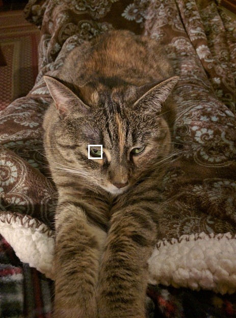
Consider this image of a cat, in particular the area of the image outlined by the white square.
Now, zoom in on the area of the cat’s eye, as shown in the left-hand image below. When we apply a filter, we consider each pixel in the image, one at a time. In this example, the pixel we are currently working on is highlighted in red, as shown in the right-hand image.
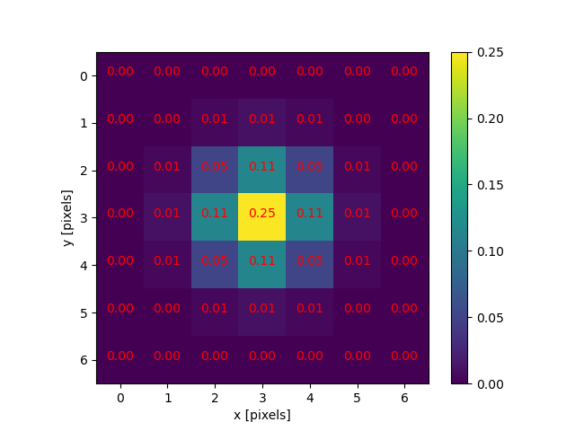
When we apply a filter, we consider rectangular groups of pixels surrounding each pixel in the image, in turn. The kernel is another group of pixels (a separate matrix / small image), of the same dimensions as the rectangular group of pixels in the image, that moves along with the pixel being worked on by the filter. The width and height of the kernel must be an odd number, so that the pixel being worked on is always in its centre. In the example shown above, the kernel is square, with a dimension of seven pixels.
To apply the kernel to the current pixel, an average of the colour values of the pixels surrounding it is calculated, weighted by the values in the kernel. In a Gaussian blur, the pixels nearest the centre of the kernel are given more weight than those far away from the centre. The rate at which this weight diminishes is determined by a Gaussian function, hence the name Gaussian blur.
A Gaussian function maps random variables into a normal distribution
or “Bell Curve”. 
The shape of the function is described by a mean value μ, and a variance value σ². The mean determines the central point of the bell curve on the X axis, and the variance describes the spread of the curve.
In fact, when using Gaussian functions in Gaussian blurring, we use a 2D Gaussian function to account for X and Y dimensions, but the same rules apply. The mean μ is always 0, and represents the middle of the 2D kernel. Increasing values of σ² in either dimension increases the amount of blurring in that dimension.
The averaging is done on a channel-by-channel basis, and the average channel values become the new value for the pixel in the filtered image. Larger kernels have more values factored into the average, and this implies that a larger kernel will blur the image more than a smaller kernel.
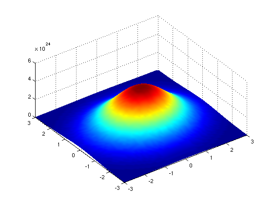
To get an idea of how this works, consider this plot of the two-dimensional Gaussian function:
Imagine that plot laid over the kernel for the Gaussian blur filter. The height of the plot corresponds to the weight given to the underlying pixel in the kernel. I.e., the pixels close to the centre become more important to the filtered pixel colour than the pixels close to the outer limits of the kernel. The shape of the Gaussian function is controlled via its standard deviation, or sigma. A large sigma value results in a flatter shape, while a smaller sigma value results in a more pronounced peak. The mathematics involved in the Gaussian blur filter are not quite that simple, but this explanation gives you the basic idea.
To illustrate the blurring process, consider the blue channel colour values from the seven-by-seven region of the cat image above:
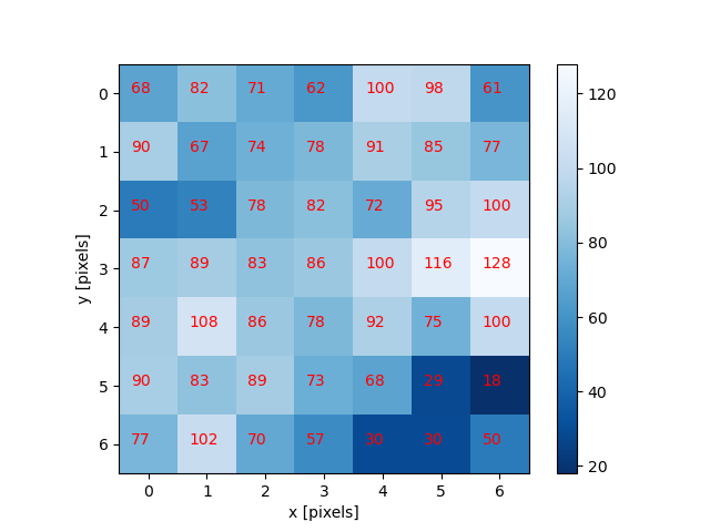
The filter is going to determine the new blue channel value for the centre pixel – the one that currently has the value 86. The filter calculates a weighted average of all the blue channel values in the kernel giving higher weight to the pixels near the centre of the kernel.
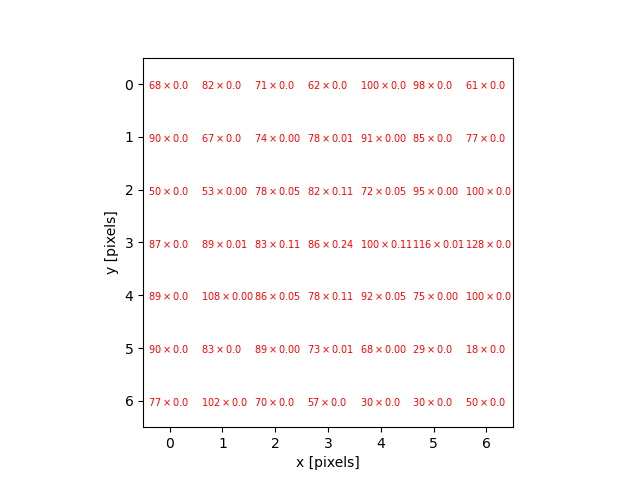
This weighted average, the sum of the multiplications, becomes the new value for the centre pixel (3, 3). The same process would be used to determine the green and red channel values, and then the kernel would be moved over to apply the filter to the next pixel in the image.
Take care to avoid mixing up the term “edge” to describe the edges of objects within an image and the outer boundaries of the images themselves. Lack of a clear distinction here may be confusing for learners.
Image edges
Something different needs to happen for pixels near the outer limits of the image, since the kernel for the filter may be partially off the image. For example, what happens when the filter is applied to the upper-left pixel of the image? Here are the blue channel pixel values for the upper-left pixel of the cat image, again assuming a seven-by-seven kernel:
OUTPUT
  x   x   x   x   x   x   x
  x   x   x   x   x   x   x
  x   x   x   x   x   x   x
  x   x   x   4   5   9   2
  x   x   x   5   3   6   7
  x   x   x   6   5   7   8
  x   x   x   5   4   5   3
The upper-left pixel is the one with value 4. Since the pixel is at the upper-left corner, there are no pixels underneath much of the kernel; here, this is represented by x’s. So, what does the filter do in that situation?
The default mode is to fill in the nearest pixel value from the image. For each of the missing x’s the image value closest to the x is used. If we fill in a few of the missing pixels, you will see how this works:
OUTPUT
  x   x   x   4   x   x   x
  x   x   x   4   x   x   x
  x   x   x   4   x   x   x
  4   4   4   4   5   9   2
  x   x   x   5   3   6   7
  x   x   x   6   5   7   8
  x   x   x   5   4   5   3
Another strategy to fill those missing values is to reflect the pixels that are in the image to fill in for the pixels that are missing from the kernel.
OUTPUT
  x   x   x   5   x   x   x
  x   x   x   6   x   x   x
  x   x   x   5   x   x   x
  2   9   5   4   5   9   2
  x   x   x   5   3   6   7
  x   x   x   6   5   7   8
  x   x   x   5   4   5   3
A similar process would be used to fill in all of the other missing pixels from the kernel. Other border modes are available; you can learn more about them in the scikit-image documentation.
This animation shows how the blur kernel moves along in the original image in order to calculate the colour channel values for the blurred image.
scikit-image has built-in functions to perform blurring for us, so we do not have to perform all of these mathematical operations ourselves. Let’s work through an example of blurring an image with the scikit-image Gaussian blur function.
First, import the packages needed for this episode:
PYTHON
import imageio.v3 as iio
import ipympl
import matplotlib.pyplot as plt
import skimage as ski

%matplotlib widget
Then, we load the image, and display it:
PYTHON
image = iio.imread(uri="data/gaussian-original.png")

# display the image
fig, ax = plt.subplots()
ax.imshow(image)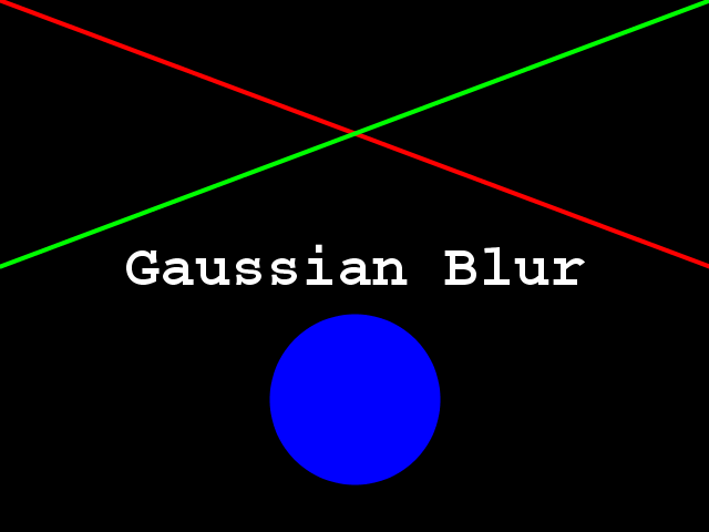
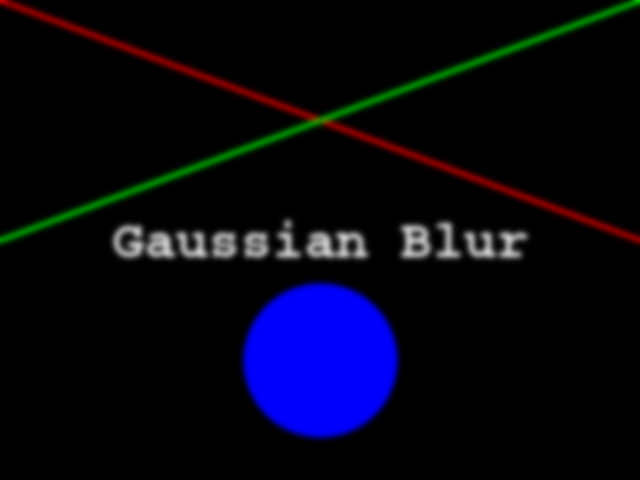
Next, we apply the gaussian blur:
PYTHON
sigma = 3.0

# apply Gaussian blur, creating a new image
blurred = ski.filters.gaussian(
    image, sigma=(sigma, sigma), truncate=3.5, channel_axis=-1)
The first two arguments to ski.filters.gaussian() are
the image to blur, image, and a tuple defining the sigma to
use in ry- and cx-direction, (sigma, sigma). The third
parameter truncate is meant to pass the radius of the
kernel in number of sigmas. A Gaussian function is defined from
-infinity to +infinity, but our kernel (which must have a finite,
smaller size) can only approximate the real function. Therefore, we must
choose a certain distance from the centre of the function where we stop
this approximation, and set the final size of our kernel. In the above
example, we set truncate to 3.5, which means the kernel
size will be 2 * sigma * 3.5. For example, for a sigma of
1.0 the resulting kernel size would be 7, while for a sigma
of 2.0 the kernel size would be 14. The default value for
truncate in scikit-image is 4.0.
The last argument we passed to ski.filters.gaussian() is
used to specify the dimension which contains the (colour) channels.
Here, it is the last dimension; recall that, in Python, the
-1 index refers to the last position. In this case, the
last dimension is the third dimension (index 2), since our
image has three dimensions:
OUTPUT
3Finally, we display the blurred image:
Visualising Blurring
Somebody said once “an image is worth a thousand words”. What is actually happening to the image pixels when we apply blurring may be difficult to grasp. Let’s now visualise the effects of blurring from a different perspective.
Let’s use the petri-dish image from previous episodes:
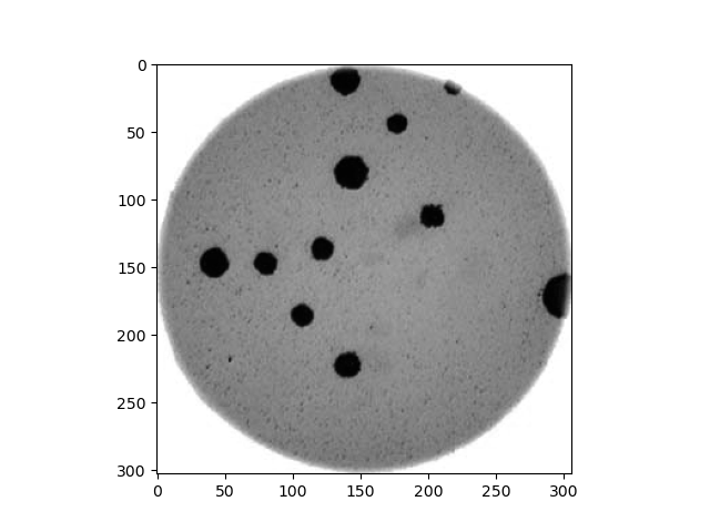
What we want to see here is the pixel intensities from a lateral
perspective: we want to see the profile of intensities. For instance,
let’s look for the intensities of the pixels along the horizontal line
at Y=150:
PYTHON
# read colonies color image and convert to grayscale
image = iio.imread('data/colonies-01.tif')
image_gray = ski.color.rgb2gray(image)
# define the pixels for which we want to view the intensity (profile)
xmin, xmax = (0, image_gray.shape[1])
Y = ymin = ymax = 150
# view the image indicating the profile pixels position
fig, ax = plt.subplots()
ax.imshow(image_gray, cmap='gray')
ax.plot([xmin, xmax], [ymin, ymax], color='red')The intensity of those pixels we can see with a simple line plot:
PYTHON
# select the vector of pixels along "Y"
image_gray_pixels_slice = image_gray[Y, :]
# guarantee the intensity values are in the [0:255] range (unsigned integers)
image_gray_pixels_slice = ski.img_as_ubyte(image_gray_pixels_slice)
fig, ax = plt.subplots()
ax.plot(image_gray_pixels_slice, color='red')
ax.set_ylim(255, 0)
ax.set_ylabel('L')
ax.set_xlabel('X')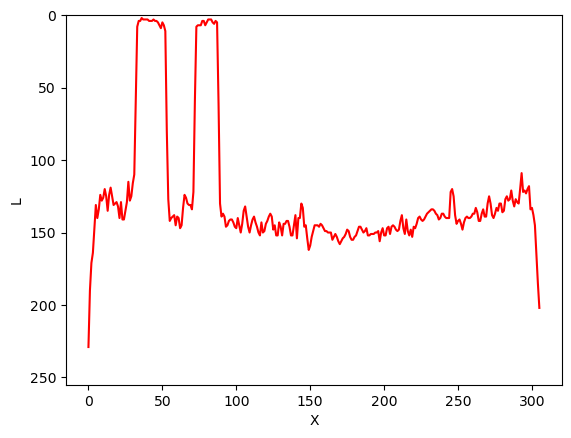
And now, how does the same set of pixels look in the corresponding blurred image:
PYTHON
# first, create a blurred version of (grayscale) image
image_blur = ski.filters.gaussian(image_gray, sigma=3)
# like before, plot the pixels profile along "Y"
image_blur_pixels_slice = image_blur[Y, :]
image_blur_pixels_slice = ski.img_as_ubyte(image_blur_pixels_slice)
fig, ax = plt.subplots()
ax.plot(image_blur_pixels_slice, 'red')
ax.set_ylim(255, 0)
ax.set_ylabel('L')
ax.set_xlabel('X')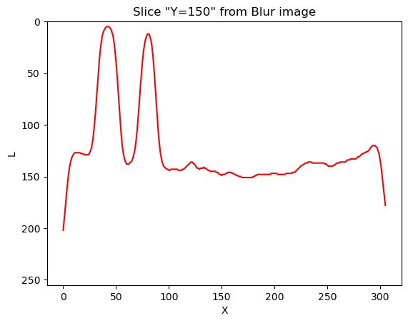
And that is why blurring is also called smoothing. This is how low-pass filters affect neighbouring pixels.
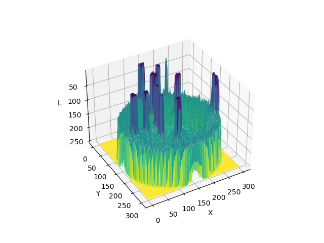
Now that we have seen the effects of blurring an image from two different perspectives, front and lateral, let’s take yet another look using a 3D visualisation.

Experimenting with sigma values (10 min)
The size and shape of the kernel used to blur an image can have a significant effect on the result of the blurring and any downstream analysis carried out on the blurred image. The next two exercises ask you to experiment with the sigma values of the kernel, which is a good way to develop your understanding of how the choice of kernel can influence the result of blurring.
First, try running the code above with a range of smaller and larger sigma values. Generally speaking, what effect does the sigma value have on the blurred image?
Generally speaking, the larger the sigma value, the more blurry the result. A larger sigma will tend to get rid of more noise in the image, which will help for other operations we will cover soon, such as thresholding. However, a larger sigma also tends to eliminate some of the detail from the image. So, we must strike a balance with the sigma value used for blur filters.
Experimenting with kernel shape (10 min - optional, not included in timing)
Now, what is the effect of applying an asymmetric kernel to blurring an image? Try running the code above with different sigmas in the ry and cx direction. For example, a sigma of 1.0 in the ry direction, and 6.0 in the cx direction.
PYTHON
# apply Gaussian blur, with a sigma of 1.0 in the ry direction, and 6.0 in the cx direction
blurred = ski.filters.gaussian(
image, sigma=(1.0, 6.0), truncate=3.5, channel_axis=-1
)
# display blurred image
fig, ax = plt.subplots()
ax.imshow(blurred)
These unequal sigma values produce a kernel that is rectangular instead of square. The result is an image that is much more blurred in the X direction than in the Y direction. For most use cases, a uniform blurring effect is desirable and this kind of asymmetric blurring should be avoided. However, it can be helpful in specific circumstances, e.g., when noise is present in your image in a particular pattern or orientation, such as vertical lines, or when you want to remove uniform noise without blurring edges present in the image in a particular orientation.
Other methods of blurring
The Gaussian blur is a way to apply a low-pass filter in
scikit-image. It is often used to remove Gaussian (i.e., random) noise
in an image. For other kinds of noise, e.g., “salt and pepper”, a median
filter is typically used. See the
skimage.filters documentation for a list of available
filters.
Key Points
- Applying a low-pass blurring filter smooths edges and removes noise from an image.
- Blurring is often used as a first step before we perform thresholding or edge detection.
- The Gaussian blur can be applied to an image with the
ski.filters.gaussian()function. - Larger sigma values may remove more noise, but they will also remove detail from an image.