Content from Background and Metadata
Last updated on 2023-05-04 | Edit this page
Overview
Questions
- What data are we using?
- Why is this experiment important?
Objectives
- Why study E. coli?
- Understand the data set.
- What is hypermutability?
Background
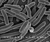
We are going to use a long-term sequencing dataset from a population of Escherichia coli.
-
What is E. coli?
- E. coli are rod-shaped bacteria that can survive under a wide variety of conditions including variable temperatures, nutrient availability, and oxygen levels. Most strains are harmless, but some are associated with food-poisoning.
-
Why is E. coli important?
- E. coli are one of the most well-studied model organisms in science. As a single-celled organism, E. coli reproduces rapidly, typically doubling its population every 20 minutes, which means it can be manipulated easily in experiments. In addition, most naturally occurring strains of E. coli are harmless. Most importantly, the genetics of E. coli are fairly well understood and can be manipulated to study adaptation and evolution.
The data
The data we are going to use is part of a long-term evolution experiment led by Richard Lenski.
The experiment was designed to assess adaptation in E. coli. A population was propagated for more than 40,000 generations in a glucose-limited minimal medium (in most conditions glucose is the best carbon source for E. coli, providing faster growth than other sugars). This medium was supplemented with citrate, which E. coli cannot metabolize in the aerobic conditions of the experiment. Sequencing of the populations at regular time points revealed that spontaneous citrate-using variant (Cit+) appeared between 31,000 and 31,500 generations, causing an increase in population size and diversity. In addition, this experiment showed hypermutability in certain regions. Hypermutability is important and can help accelerate adaptation to novel environments, but also can be selected against in well-adapted populations.
To see a timeline of the experiment to date, check out this figure, and this paper Blount et al. 2008: Historical contingency and the evolution of a key innovation in an experimental population of Escherichia coli.
View the metadata
We will be working with three sample events from the Ara-3 strain of this experiment, one from 5,000 generations, one from 15,000 generations, and one from 50,000 generations. The population changed substantially during the course of the experiment, and we will be exploring how (the evolution of a Cit+ mutant and hypermutability) with our variant calling workflow. The metadata file associated with this lesson can be downloaded directly here or viewed in Github. If you would like to know details of how the file was created, you can look at some notes and sources here.
This metadata describes information on the Ara-3 clones and the columns represent:
| Column | Description |
|---|---|
| strain | strain name |
| generation | generation when sample frozen |
| clade | based on parsimony-based tree |
| reference | study the samples were originally sequenced for |
| population | ancestral population group |
| mutator | hypermutability mutant status |
| facility | facility samples were sequenced at |
| run | Sequence read archive sample ID |
| read_type | library type of reads |
| read_length | length of reads in sample |
| sequencing_depth | depth of sequencing |
| cit | citrate-using mutant status |
Challenge
Based on the metadata, can you answer the following questions?
- How many different generations exist in the data?
- How many rows and how many columns are in this data?
- How many citrate+ mutants have been recorded in Ara-3?
- How many hypermutable mutants have been recorded in Ara-3?
- 25 different generations
- 62 rows, 12 columns
- 10 citrate+ mutants
- 6 hypermutable mutants
Key Points
- It is important to record and understand your experiment’s metadata.
Content from Assessing Read Quality
Last updated on 2023-05-04 | Edit this page
Overview
Questions
- How can I describe the quality of my data?
Objectives
- Explain how a FASTQ file encodes per-base quality scores.
- Interpret a FastQC plot summarizing per-base quality across all reads.
- Use
forloops to automate operations on multiple files.
Bioinformatic workflows
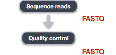
When working with high-throughput sequencing data, the raw reads you get off of the sequencer will need to pass through a number of different tools in order to generate your final desired output. The execution of this set of tools in a specified order is commonly referred to as a workflow or a pipeline.
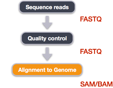
An example of the workflow we will be using for our variant calling analysis is provided below with a brief description of each step.
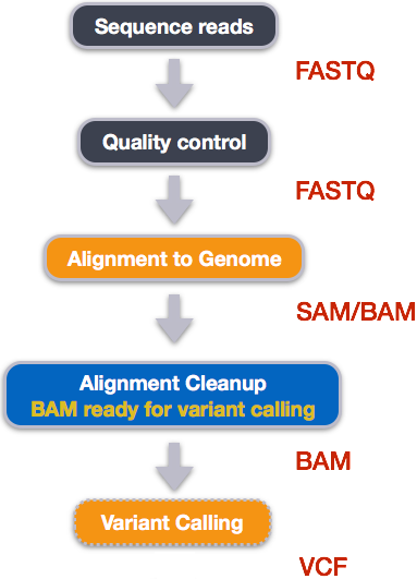
- Quality control - Assessing quality using FastQC
- Quality control - Trimming and/or filtering reads (if necessary)
- Align reads to reference genome
- Perform post-alignment clean-up
- Variant calling
These workflows in bioinformatics adopt a plug-and-play approach in that the output of one tool can be easily used as input to another tool without any extensive configuration. Having standards for data formats is what makes this feasible. Standards ensure that data is stored in a way that is generally accepted and agreed upon within the community. The tools that are used to analyze data at different stages of the workflow are therefore built under the assumption that the data will be provided in a specific format.
Starting with data
Often times, the first step in a bioinformatic workflow is getting the data you want to work with onto a computer where you can work with it. If you have outsourced sequencing of your data, the sequencing center will usually provide you with a link that you can use to download your data. Today we will be working with publicly available sequencing data.
We are studying a population of Escherichia coli (designated Ara-3), which were propagated for more than 50,000 generations in a glucose-limited minimal medium. We will be working with three samples from this experiment, one from 5,000 generations, one from 15,000 generations, and one from 50,000 generations. The population changed substantially during the course of the experiment, and we will be exploring how with our variant calling workflow.
The data are paired-end, so we will download two files for each sample. We will use the European Nucleotide Archive to get our data. The ENA “provides a comprehensive record of the world’s nucleotide sequencing information, covering raw sequencing data, sequence assembly information and functional annotation.” The ENA also provides sequencing data in the fastq format, an important format for sequencing reads that we will be learning about today.
To download the data, run the commands below.
Here we are using the -p option for mkdir.
This option allows mkdir to create the new directory, even
if one of the parent directories does not already exist. It also
supresses errors if the directory already exists, without overwriting
that directory.
It will take about 15 minutes to download the files.
BASH
mkdir -p ~/dc_workshop/data/untrimmed_fastq/
cd ~/dc_workshop/data/untrimmed_fastq

curl -O ftp://ftp.sra.ebi.ac.uk/vol1/fastq/SRR258/004/SRR2589044/SRR2589044_1.fastq.gz
curl -O ftp://ftp.sra.ebi.ac.uk/vol1/fastq/SRR258/004/SRR2589044/SRR2589044_2.fastq.gz
curl -O ftp://ftp.sra.ebi.ac.uk/vol1/fastq/SRR258/003/SRR2584863/SRR2584863_1.fastq.gz
curl -O ftp://ftp.sra.ebi.ac.uk/vol1/fastq/SRR258/003/SRR2584863/SRR2584863_2.fastq.gz
curl -O ftp://ftp.sra.ebi.ac.uk/vol1/fastq/SRR258/006/SRR2584866/SRR2584866_1.fastq.gz
curl -O ftp://ftp.sra.ebi.ac.uk/vol1/fastq/SRR258/006/SRR2584866/SRR2584866_2.fastq.gz
Faster option
If your workshop is short on time or the venue’s internet connection
is weak or unstable, learners can avoid needing to download the data and
instead use the data files provided in the .backup/
directory.
This command creates a copy of each of the files in the
.backup/untrimmed_fastq/ directory that end in
fastq.gz and places the copies in the current working
directory (signified by .).
The data comes in a compressed format, which is why there is a
.gz at the end of the file names. This makes it faster to
transfer, and allows it to take up less space on our computer. Let’s
unzip one of the files so that we can look at the fastq format.
Quality control
We will now assess the quality of the sequence reads contained in our fastq files.
Details on the FASTQ format
Although it looks complicated (and it is), we can understand the fastq format with a little decoding. Some rules about the format include…
| Line | Description |
|---|---|
| 1 | Always begins with ‘@’ and then information about the read |
| 2 | The actual DNA sequence |
| 3 | Always begins with a ‘+’ and sometimes the same info in line 1 |
| 4 | Has a string of characters which represent the quality scores; must have same number of characters as line 2 |
We can view the first complete read in one of the files our dataset
by using head to look at the first four lines.
OUTPUT
@SRR2584863.1 HWI-ST957:244:H73TDADXX:1:1101:4712:2181/1
TTCACATCCTGACCATTCAGTTGAGCAAAATAGTTCTTCAGTGCCTGTTTAACCGAGTCACGCAGGGGTTTTTGGGTTACCTGATCCTGAGAGTTAACGGTAGAAACGGTCAGTACGTCAGAATTTACGCGTTGTTCGAACATAGTTCTG
+
CCCFFFFFGHHHHJIJJJJIJJJIIJJJJIIIJJGFIIIJEDDFEGGJIFHHJIJJDECCGGEGIIJFHFFFACD:BBBDDACCCCAA@@CA@C>C3>@5(8&>C:9?8+89<4(:83825C(:A#########################
Line 4 shows the quality for each nucleotide in the read. Quality is interpreted as the probability of an incorrect base call (e.g. 1 in 10) or, equivalently, the base call accuracy (e.g. 90%). To make it possible to line up each individual nucleotide with its quality score, the numerical score is converted into a code where each individual character represents the numerical quality score for an individual nucleotide. For example, in the line above, the quality score line is:
OUTPUT
CCCFFFFFGHHHHJIJJJJIJJJIIJJJJIIIJJGFIIIJEDDFEGGJIFHHJIJJDECCGGEGIIJFHFFFACD:BBBDDACCCCAA@@CA@C>C3>@5(8&>C:9?8+89<4(:83825C(:A#########################The numerical value assigned to each of these characters depends on the sequencing platform that generated the reads. The sequencing machine used to generate our data uses the standard Sanger quality PHRED score encoding, using Illumina version 1.8 onwards. Each character is assigned a quality score between 0 and 41 as shown in the chart below.
OUTPUT
Quality encoding: !"#$%&'()*+,-./0123456789:;<=>?@ABCDEFGHIJ
                   |         |         |         |         |
Quality score:    01........11........21........31........41
Each quality score represents the probability that the corresponding nucleotide call is incorrect. This quality score is logarithmically based, so a quality score of 10 reflects a base call accuracy of 90%, but a quality score of 20 reflects a base call accuracy of 99%. These probability values are the results from the base calling algorithm and depend on how much signal was captured for the base incorporation.
Looking back at our read:
OUTPUT
@SRR2584863.1 HWI-ST957:244:H73TDADXX:1:1101:4712:2181/1
TTCACATCCTGACCATTCAGTTGAGCAAAATAGTTCTTCAGTGCCTGTTTAACCGAGTCACGCAGGGGTTTTTGGGTTACCTGATCCTGAGAGTTAACGGTAGAAACGGTCAGTACGTCAGAATTTACGCGTTGTTCGAACATAGTTCTG
+
CCCFFFFFGHHHHJIJJJJIJJJIIJJJJIIIJJGFIIIJEDDFEGGJIFHHJIJJDECCGGEGIIJFHFFFACD:BBBDDACCCCAA@@CA@C>C3>@5(8&>C:9?8+89<4(:83825C(:A#########################
we can now see that there is a range of quality scores, but that the
end of the sequence is very poor (# = a quality score of
2).
Exercise
What is the last read in the SRR2584863_1.fastq file?
How confident are you in this read?
OUTPUT
@SRR2584863.1553259 HWI-ST957:245:H73R4ADXX:2:2216:21048:100894/1
CTGCAATACCACGCTGATCTTTCACATGATGTAAGAAAAGTGGGATCAGCAAACCGGGTGCTGCTGTGGCTAGTTGCAGCAAACCATGCAGTGAACCCGCCTGTGCTTCGCTATAGCCGTGACTGATGAGGATCGCCGGAAGCCAGCCAA
+
CCCFFFFFHHHHGJJJJJJJJJHGIJJJIJJJJIJJJJIIIIJJJJJJJJJJJJJIIJJJHHHHHFFFFFEEEEEDDDDDDDDDDDDDDDDDCDEDDBDBDDBDDDDDDDDDBDEEDDDD7@BDDDDDD>AA>?B?<@BDD@BDC?BDA?
This read has more consistent quality at its end than the first read that we looked at, but still has a range of quality scores, most of them high. We will look at variations in position-based quality in just a moment.
At this point, lets validate that all the relevant tools are installed. If you are using the AWS AMI then these should be preinstalled.
BASH
$ fastqc -h
            FastQC - A high throughput sequence QC analysis tool

SYNOPSIS

        fastqc seqfile1 seqfile2 .. seqfileN

    fastqc [-o output dir] [--(no)extract] [-f fastq|bam|sam]
           [-c contaminant file] seqfile1 .. seqfileN

DESCRIPTION

    FastQC reads a set of sequence files and produces from each one a quality
    control report consisting of a number of different modules, each one of
    which will help to identify a different potential type of problem in your
    data.

    If no files to process are specified on the command line then the program
    will start as an interactive graphical application.  If files are provided
    on the command line then the program will run with no user interaction
    required.  In this mode it is suitable for inclusion into a standardised
    analysis pipeline.

    The options for the program as as follows:

    -h --help       Print this help file and exit

    -v --version    Print the version of the program and exit

    -o --outdir     Create all output files in the specified output directory.
                    Please note that this directory must exist as the program
                    will not create it.  If this option is not set then the
                    output file for each sequence file is created in the same
                    directory as the sequence file which was processed.

    --casava        Files come from raw casava output. Files in the same sample
                    group (differing only by the group number) will be analysed
                    as a set rather than individually. Sequences with the filter
                    flag set in the header will be excluded from the analysis.
                    Files must have the same names given to them by casava
                    (including being gzipped and ending with .gz) otherwise they
                    will not be grouped together correctly.

    --nano          Files come from naopore sequences and are in fast5 format. In
                    this mode you can pass in directories to process and the program
                    will take in all fast5 files within those directories and produce
                    a single output file from the sequences found in all files.

    --nofilter      If running with --casava then don't remove read flagged by
                    casava as poor quality when performing the QC analysis.

    --extract       If set then the zipped output file will be uncompressed in
                    the same directory after it has been created.  By default
                    this option will be set if fastqc is run in non-interactive
                    mode.

    -j --java       Provides the full path to the java binary you want to use to
                    launch fastqc. If not supplied then java is assumed to be in
                    your path.

    --noextract     Do not uncompress the output file after creating it.  You
                    should set this option if you do not wish to uncompress
                    the output when running in non-interactive mode.

    --nogroup       Disable grouping of bases for reads >50bp. All reports will
                    show data for every base in the read.  WARNING: Using this
                    option will cause fastqc to crash and burn if you use it on
                    really long reads, and your plots may end up a ridiculous size.
                    You have been warned!

    -f --format     Bypasses the normal sequence file format detection and
                    forces the program to use the specified format.  Valid
                    formats are bam,sam,bam_mapped,sam_mapped and fastq

    -t --threads    Specifies the number of files which can be processed
                    simultaneously.  Each thread will be allocated 250MB of
                    memory so you shouldn't run more threads than your
                    available memory will cope with, and not more than
                    6 threads on a 32 bit machine

    -c              Specifies a non-default file which contains the list of
    --contaminants  contaminants to screen overrepresented sequences against.
                    The file must contain sets of named contaminants in the
                    form name[tab]sequence.  Lines prefixed with a hash will
                    be ignored.

    -a              Specifies a non-default file which contains the list of
    --adapters      adapter sequences which will be explicity searched against
                    the library. The file must contain sets of named adapters
                    in the form name[tab]sequence.  Lines prefixed with a hash
                    will be ignored.

    -l              Specifies a non-default file which contains a set of criteria
    --limits        which will be used to determine the warn/error limits for the
                    various modules.  This file can also be used to selectively
                    remove some modules from the output all together.  The format
                    needs to mirror the default limits.txt file found in the
                    Configuration folder.

   -k --kmers       Specifies the length of Kmer to look for in the Kmer content
                    module. Specified Kmer length must be between 2 and 10. Default
                    length is 7 if not specified.

   -q --quiet       Supress all progress messages on stdout and only report errors.

   -d --dir         Selects a directory to be used for temporary files written when
                    generating report images. Defaults to system temp directory if
                    not specified.

BUGS

    Any bugs in fastqc should be reported either to simon.andrews@babraham.ac.uk
    or in www.bioinformatics.babraham.ac.uk/bugzilla/
if fastqc is not installed then you would expect to see an error like
$ fastqc -h
The program 'fastqc' is currently not installed. You can install it by typing:
sudo apt-get install fastqc
If this happens check with your instructor before trying to install it.
Assessing quality using FastQC
In real life, you will not be assessing the quality of your reads by visually inspecting your FASTQ files. Rather, you will be using a software program to assess read quality and filter out poor quality reads. We will first use a program called FastQC to visualize the quality of our reads. Later in our workflow, we will use another program to filter out poor quality reads.
FastQC has a number of features which can give you a quick impression of any problems your data may have, so you can take these issues into consideration before moving forward with your analyses. Rather than looking at quality scores for each individual read, FastQC looks at quality collectively across all reads within a sample. The image below shows one FastQC-generated plot that indicates a very high quality sample:
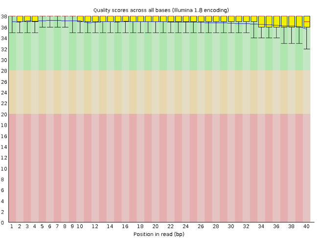
The x-axis displays the base position in the read, and the y-axis shows quality scores. In this example, the sample contains reads that are 40 bp long. This is much shorter than the reads we are working with in our workflow. For each position, there is a box-and-whisker plot showing the distribution of quality scores for all reads at that position. The horizontal red line indicates the median quality score and the yellow box shows the 1st to 3rd quartile range. This means that 50% of reads have a quality score that falls within the range of the yellow box at that position. The whiskers show the absolute range, which covers the lowest (0th quartile) to highest (4th quartile) values.
For each position in this sample, the quality values do not drop much lower than 32. This is a high quality score. The plot background is also color-coded to identify good (green), acceptable (yellow), and bad (red) quality scores.
Now let’s take a look at a quality plot on the other end of the spectrum.
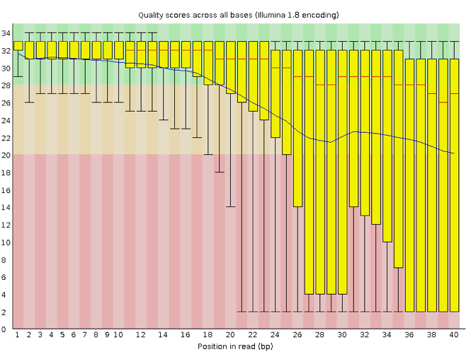
Here, we see positions within the read in which the boxes span a much wider range. Also, quality scores drop quite low into the “bad” range, particularly on the tail end of the reads. The FastQC tool produces several other diagnostic plots to assess sample quality, in addition to the one plotted above.
Running FastQC
We will now assess the quality of the reads that we downloaded.
First, make sure you are still in the untrimmed_fastq
directory
Exercise
How big are the files? (Hint: Look at the options for the
ls command to see how to show file sizes.)
OUTPUT
-rw-rw-r-- 1 dcuser dcuser 545M Jul  6 20:27 SRR2584863_1.fastq
-rw-rw-r-- 1 dcuser dcuser 183M Jul  6 20:29 SRR2584863_2.fastq.gz
-rw-rw-r-- 1 dcuser dcuser 309M Jul  6 20:34 SRR2584866_1.fastq.gz
-rw-rw-r-- 1 dcuser dcuser 296M Jul  6 20:37 SRR2584866_2.fastq.gz
-rw-rw-r-- 1 dcuser dcuser 124M Jul  6 20:22 SRR2589044_1.fastq.gz
-rw-rw-r-- 1 dcuser dcuser 128M Jul  6 20:24 SRR2589044_2.fastq.gz
There are six FASTQ files ranging from 124M (124MB) to 545M.
FastQC can accept multiple file names as input, and on both zipped and unzipped files, so we can use the *.fastq* wildcard to run FastQC on all of the FASTQ files in this directory.
You will see an automatically updating output message telling you the progress of the analysis. It will start like this:
OUTPUT
Started analysis of SRR2584863_1.fastq
Approx 5% complete for SRR2584863_1.fastq
Approx 10% complete for SRR2584863_1.fastq
Approx 15% complete for SRR2584863_1.fastq
Approx 20% complete for SRR2584863_1.fastq
Approx 25% complete for SRR2584863_1.fastq
Approx 30% complete for SRR2584863_1.fastq
Approx 35% complete for SRR2584863_1.fastq
Approx 40% complete for SRR2584863_1.fastq
Approx 45% complete for SRR2584863_1.fastq
In total, it should take about five minutes for FastQC to run on all six of our FASTQ files. When the analysis completes, your prompt will return. So your screen will look something like this:
OUTPUT
Approx 80% complete for SRR2589044_2.fastq.gz
Approx 85% complete for SRR2589044_2.fastq.gz
Approx 90% complete for SRR2589044_2.fastq.gz
Approx 95% complete for SRR2589044_2.fastq.gz
Analysis complete for SRR2589044_2.fastq.gz
$
The FastQC program has created several new files within our
data/untrimmed_fastq/ directory.
OUTPUT
SRR2584863_1.fastq        SRR2584866_1_fastqc.html  SRR2589044_1_fastqc.html
SRR2584863_1_fastqc.html  SRR2584866_1_fastqc.zip   SRR2589044_1_fastqc.zip
SRR2584863_1_fastqc.zip   SRR2584866_1.fastq.gz     SRR2589044_1.fastq.gz
SRR2584863_2_fastqc.html  SRR2584866_2_fastqc.html  SRR2589044_2_fastqc.html
SRR2584863_2_fastqc.zip   SRR2584866_2_fastqc.zip   SRR2589044_2_fastqc.zip
SRR2584863_2.fastq.gz     SRR2584866_2.fastq.gz     SRR2589044_2.fastq.gz
For each input FASTQ file, FastQC has created a .zip
file and a
.html file. The .zip file extension
indicates that this is actually a compressed set of multiple output
files. We will be working with these output files soon. The
.html file is a stable webpage displaying the summary
report for each of our samples.
We want to keep our data files and our results files separate, so we
will move these output files into a new directory within our
results/ directory.
BASH
$ mkdir -p ~/dc_workshop/results/fastqc_untrimmed_reads
$ mv *.zip ~/dc_workshop/results/fastqc_untrimmed_reads/
$ mv *.html ~/dc_workshop/results/fastqc_untrimmed_reads/
Now we can navigate into this results directory and do some closer inspection of our output files.
Viewing the FastQC results
If we were working on our local computers, we would be able to look at each of these HTML files by opening them in a web browser.
However, these files are currently sitting on our remote AWS instance, where our local computer can not see them. And, since we are only logging into the AWS instance via the command line - it does not have any web browser setup to display these files either.
So the easiest way to look at these webpage summary reports will be to transfer them to our local computers (i.e. your laptop).
To transfer a file from a remote server to our own machines, we will
use scp, which we learned yesterday in the Shell Genomics
lesson.
First we will make a new directory on our computer to store the HTML files we are transferring. Let’s put it on our desktop for now. Open a new tab in your terminal program (you can use the pull down menu at the top of your screen or the Cmd+t keyboard shortcut) and type:
Now we can transfer our HTML files to our local computer using
scp.
BASH
$ scp dcuser@ec2-34-238-162-94.compute-1.amazonaws.com:~/dc_workshop/results/fastqc_untrimmed_reads/*.html ~/Desktop/fastqc_htmlNote on using zsh
If you are using zsh instead of bash (macOS for example changed the
default recently to zsh), it is likely that a
no matches found error will be displayed. The reason for
this is that the wildcard (“*”) is not correctly interpreted. To fix
this problem the wildcard needs to be escaped with a “\”:
BASH
$ scp dcuser@ec2-34-238-162-94.compute-1.amazonaws.com:~/dc_workshop/results/fastqc_untrimmed_reads/\*.html ~/Desktop/fastqc_htmlAlternatively, you can put the whole path into quotation marks:
As a reminder, the first part of the command
dcuser@ec2-34-238-162-94.compute-1.amazonaws.com is the
address for your remote computer. Make sure you replace everything after
dcuser@ with your instance number (the one you used to log
in).
The second part starts with a : and then gives the
absolute path of the files you want to transfer from your remote
computer. Do not forget the :. We used a wildcard
(*.html) to indicate that we want all of the HTML
files.
The third part of the command gives the absolute path of the location
you want to put the files. This is on your local computer and is the
directory we just created ~/Desktop/fastqc_html.
You should see a status output like this:
OUTPUT
SRR2584863_1_fastqc.html                      100%  249KB 152.3KB/s   00:01
SRR2584863_2_fastqc.html                      100%  254KB 219.8KB/s   00:01
SRR2584866_1_fastqc.html                      100%  254KB 271.8KB/s   00:00
SRR2584866_2_fastqc.html                      100%  251KB 252.8KB/s   00:00
SRR2589044_1_fastqc.html                      100%  249KB 370.1KB/s   00:00
SRR2589044_2_fastqc.html                      100%  251KB 592.2KB/s   00:00
Now we can go to our new directory and open the 6 HTML files.
Depending on your system, you should be able to select and open them all at once via a right click menu in your file browser.
Exercise
Discuss your results with a neighbor. Which sample(s) looks the best in terms of per base sequence quality? Which sample(s) look the worst?
All of the reads contain usable data, but the quality decreases toward the end of the reads.
Decoding the other FastQC outputs
We have now looked at quite a few “Per base sequence quality” FastQC graphs, but there are nine other graphs that we have not talked about! Below we have provided a brief overview of interpretations for each of these plots. For more information, please see the FastQC documentation here
- Per tile sequence quality: the machines that perform sequencing are divided into tiles. This plot displays patterns in base quality along these tiles. Consistently low scores are often found around the edges, but hot spots can also occur in the middle if an air bubble was introduced at some point during the run.
- Per sequence quality scores: a density plot of quality for all reads at all positions. This plot shows what quality scores are most common.
- Per base sequence content: plots the proportion of each base position over all of the reads. Typically, we expect to see each base roughly 25% of the time at each position, but this often fails at the beginning or end of the read due to quality or adapter content.
- Per sequence GC content: a density plot of average GC content in each of the reads.
- Per base N content: the percent of times that ‘N’ occurs at a position in all reads. If there is an increase at a particular position, this might indicate that something went wrong during sequencing.
- Sequence Length Distribution: the distribution of sequence lengths of all reads in the file. If the data is raw, there is often on sharp peak, however if the reads have been trimmed, there may be a distribution of shorter lengths.
- Sequence Duplication Levels: A distribution of duplicated sequences. In sequencing, we expect most reads to only occur once. If some sequences are occurring more than once, it might indicate enrichment bias (e.g. from PCR). If the samples are high coverage (or RNA-seq or amplicon), this might not be true.
- Overrepresented sequences: A list of sequences that occur more frequently than would be expected by chance.
- Adapter Content: a graph indicating where adapater sequences occur in the reads.
- K-mer Content: a graph showing any sequences which may show a positional bias within the reads.
Working with the FastQC text output
Now that we have looked at our HTML reports to get a feel for the
data, let’s look more closely at the other output files. Go back to the
tab in your terminal program that is connected to your AWS instance (the
tab label will start with dcuser@ip) and make sure you are
in our results subdirectory.
OUTPUT
SRR2584863_1_fastqc.html  SRR2584866_1_fastqc.html  SRR2589044_1_fastqc.html
SRR2584863_1_fastqc.zip   SRR2584866_1_fastqc.zip   SRR2589044_1_fastqc.zip
SRR2584863_2_fastqc.html  SRR2584866_2_fastqc.html  SRR2589044_2_fastqc.html
SRR2584863_2_fastqc.zip   SRR2584866_2_fastqc.zip   SRR2589044_2_fastqc.zip
Our .zip files are compressed files. They each contain
multiple different types of output files for a single input FASTQ file.
To view the contents of a .zip file, we can use the program
unzip to decompress these files. Let’s try doing them all
at once using a wildcard.
OUTPUT
Archive:  SRR2584863_1_fastqc.zip
caution: filename not matched:  SRR2584863_2_fastqc.zip
caution: filename not matched:  SRR2584866_1_fastqc.zip
caution: filename not matched:  SRR2584866_2_fastqc.zip
caution: filename not matched:  SRR2589044_1_fastqc.zip
caution: filename not matched:  SRR2589044_2_fastqc.zip
This did not work. We unzipped the first file and then got a warning
message for each of the other .zip files. This is because
unzip expects to get only one zip file as input. We could
go through and unzip each file one at a time, but this is very time
consuming and error-prone. Someday you may have 500 files to unzip!
A more efficient way is to use a for loop like we
learned in the Shell Genomics lesson to iterate through all of our
.zip files. Let’s see what that looks like and then we will
discuss what we are doing with each line of our loop.
In this example, the input is six filenames (one filename for each of
our .zip files). Each time the loop iterates, it will
assign a file name to the variable filename and run the
unzip command. The first time through the loop,
$filename is SRR2584863_1_fastqc.zip. The
interpreter runs the command unzip on
SRR2584863_1_fastqc.zip. For the second iteration,
$filename becomes SRR2584863_2_fastqc.zip.
This time, the shell runs unzip on
SRR2584863_2_fastqc.zip. It then repeats this process for
the four other .zip files in our directory.
When we run our for loop, you will see output that
starts like this:
OUTPUT
Archive:  SRR2589044_2_fastqc.zip
   creating: SRR2589044_2_fastqc/
   creating: SRR2589044_2_fastqc/Icons/
   creating: SRR2589044_2_fastqc/Images/
  inflating: SRR2589044_2_fastqc/Icons/fastqc_icon.png
  inflating: SRR2589044_2_fastqc/Icons/warning.png
  inflating: SRR2589044_2_fastqc/Icons/error.png
  inflating: SRR2589044_2_fastqc/Icons/tick.png
  inflating: SRR2589044_2_fastqc/summary.txt
  inflating: SRR2589044_2_fastqc/Images/per_base_quality.png
  inflating: SRR2589044_2_fastqc/Images/per_tile_quality.png
  inflating: SRR2589044_2_fastqc/Images/per_sequence_quality.png
  inflating: SRR2589044_2_fastqc/Images/per_base_sequence_content.png
  inflating: SRR2589044_2_fastqc/Images/per_sequence_gc_content.png
  inflating: SRR2589044_2_fastqc/Images/per_base_n_content.png
  inflating: SRR2589044_2_fastqc/Images/sequence_length_distribution.png
  inflating: SRR2589044_2_fastqc/Images/duplication_levels.png
  inflating: SRR2589044_2_fastqc/Images/adapter_content.png
  inflating: SRR2589044_2_fastqc/fastqc_report.html
  inflating: SRR2589044_2_fastqc/fastqc_data.txt
  inflating: SRR2589044_2_fastqc/fastqc.fo
The unzip program is decompressing the .zip
files and creating a new directory (with subdirectories) for each of our
samples, to store all of the different output that is produced by
FastQC. There
are a lot of files here. The one we are going to focus on is the
summary.txt file.
If you list the files in our directory now you will see:
SRR2584863_1_fastqc       SRR2584866_1_fastqc       SRR2589044_1_fastqc
SRR2584863_1_fastqc.html  SRR2584866_1_fastqc.html  SRR2589044_1_fastqc.html
SRR2584863_1_fastqc.zip   SRR2584866_1_fastqc.zip   SRR2589044_1_fastqc.zip
SRR2584863_2_fastqc       SRR2584866_2_fastqc       SRR2589044_2_fastqc
SRR2584863_2_fastqc.html  SRR2584866_2_fastqc.html  SRR2589044_2_fastqc.html
SRR2584863_2_fastqc.zip   SRR2584866_2_fastqc.zip   SRR2589044_2_fastqc.zip
{:. output}
The .html files and the uncompressed .zip
files are still present, but now we also have a new directory for each
of our samples. We can see for sure that it is a directory if we use the
-F flag for ls.
OUTPUT
SRR2584863_1_fastqc/      SRR2584866_1_fastqc/      SRR2589044_1_fastqc/
SRR2584863_1_fastqc.html  SRR2584866_1_fastqc.html  SRR2589044_1_fastqc.html
SRR2584863_1_fastqc.zip   SRR2584866_1_fastqc.zip   SRR2589044_1_fastqc.zip
SRR2584863_2_fastqc/      SRR2584866_2_fastqc/      SRR2589044_2_fastqc/
SRR2584863_2_fastqc.html  SRR2584866_2_fastqc.html  SRR2589044_2_fastqc.html
SRR2584863_2_fastqc.zip   SRR2584866_2_fastqc.zip   SRR2589044_2_fastqc.zip
Let’s see what files are present within one of these output directories.
OUTPUT
fastqc_data.txt fastqc.fo fastqc_report.html Icons/ Images/ summary.txtUse less to preview the summary.txt file
for this sample.
OUTPUT
PASS    Basic Statistics        SRR2584863_1.fastq
PASS    Per base sequence quality       SRR2584863_1.fastq
PASS    Per tile sequence quality       SRR2584863_1.fastq
PASS    Per sequence quality scores     SRR2584863_1.fastq
WARN    Per base sequence content       SRR2584863_1.fastq
WARN    Per sequence GC content SRR2584863_1.fastq
PASS    Per base N content      SRR2584863_1.fastq
PASS    Sequence Length Distribution    SRR2584863_1.fastq
PASS    Sequence Duplication Levels     SRR2584863_1.fastq
PASS    Overrepresented sequences       SRR2584863_1.fastq
WARN    Adapter Content SRR2584863_1.fastq
The summary file gives us a list of tests that FastQC ran, and tells
us whether this sample passed, failed, or is borderline
(WARN). Remember, to quit from less you must
type q.
Documenting our work
We can make a record of the results we obtained for all our samples
by concatenating all of our summary.txt files into a
single file using the cat command. We will call this
fastqc_summaries.txt and move it to
~/dc_workshop/docs.
Exercise
Which samples failed at least one of FastQC’s quality tests? What test(s) did those samples fail?
We can get the list of all failed tests using grep.
OUTPUT
FAIL    Per base sequence quality       SRR2584863_2.fastq.gz
FAIL    Per tile sequence quality       SRR2584863_2.fastq.gz
FAIL    Per base sequence content       SRR2584863_2.fastq.gz
FAIL    Per base sequence quality       SRR2584866_1.fastq.gz
FAIL    Per base sequence content       SRR2584866_1.fastq.gz
FAIL    Adapter Content SRR2584866_1.fastq.gz
FAIL    Adapter Content SRR2584866_2.fastq.gz
FAIL    Adapter Content SRR2589044_1.fastq.gz
FAIL    Per base sequence quality       SRR2589044_2.fastq.gz
FAIL    Per tile sequence quality       SRR2589044_2.fastq.gz
FAIL    Per base sequence content       SRR2589044_2.fastq.gz
FAIL    Adapter Content SRR2589044_2.fastq.gz
Other notes – optional
Quality encodings vary
Although we have used a particular quality encoding system to
demonstrate interpretation of read quality, different sequencing
machines use different encoding systems. This means that, depending on
which sequencer you use to generate your data, a # may not
be an indicator of a poor quality base call.
This mainly relates to older Solexa/Illumina data, but it is essential that you know which sequencing platform was used to generate your data, so that you can tell your quality control program which encoding to use. If you choose the wrong encoding, you run the risk of throwing away good reads or (even worse) not throwing away bad reads!
Same symbols, different meanings
Here we see > being used as a shell prompt, whereas
> is also used to redirect output. Similarly,
$ is used as a shell prompt, but, as we saw earlier, it is
also used to ask the shell to get the value of a variable.
If the shell prints > or $ then
it expects you to type something, and the symbol is a prompt.
If you type > or $ yourself, it
is an instruction from you that the shell should redirect output or get
the value of a variable.
Key Points
- Quality encodings vary across sequencing platforms.
-
forloops let you perform the same set of operations on multiple files with a single command.
Content from Trimming and Filtering
Last updated on 2023-05-04 | Edit this page
Overview
Questions
- How can I get rid of sequence data that does not meet my quality standards?
Objectives
- Clean FASTQ reads using Trimmomatic.
- Select and set multiple options for command-line bioinformatic tools.
- Write
forloops with two variables.
Cleaning reads
In the previous episode, we took a high-level look at the quality of each of our samples using FastQC. We visualized per-base quality graphs showing the distribution of read quality at each base across all reads in a sample and extracted information about which samples fail which quality checks. Some of our samples failed quite a few quality metrics used by FastQC. This does not mean, though, that our samples should be thrown out! It is very common to have some quality metrics fail, and this may or may not be a problem for your downstream application. For our variant calling workflow, we will be removing some of the low quality sequences to reduce our false positive rate due to sequencing error.
We will use a program called Trimmomatic to filter poor quality reads and trim poor quality bases from our samples.
Trimmomatic options
Trimmomatic has a variety of options to trim your reads. If we run the following command, we can see some of our options.
Which will give you the following output:
OUTPUT
Usage:
       PE [-version] [-threads <threads>] [-phred33|-phred64] [-trimlog <trimLogFile>] [-summary <statsSummaryFile>] [-quiet] [-validatePairs] [-basein <inputBase> | <inputFile1> <inputFile2>] [-baseout <outputBase> | <outputFile1P> <outputFile1U> <outputFile2P> <outputFile2U>] <trimmer1>...
   or:
       SE [-version] [-threads <threads>] [-phred33|-phred64] [-trimlog <trimLogFile>] [-summary <statsSummaryFile>] [-quiet] <inputFile> <outputFile> <trimmer1>...
   or:
       -version
This output shows us that we must first specify whether we have
paired end (PE) or single end (SE) reads.
Next, we specify what flag we would like to run. For example, you can
specify threads to indicate the number of processors on
your computer that you want Trimmomatic to use. In most cases using
multiple threads (processors) can help to run the trimming faster. These
flags are not necessary, but they can give you more control over the
command. The flags are followed by positional arguments, meaning the
order in which you specify them is important. In paired end mode,
Trimmomatic expects the two input files, and then the names of the
output files. These files are described below. While, in single end
mode, Trimmomatic will expect 1 file as input, after which you can enter
the optional settings and lastly the name of the output file.
| option | meaning |
|---|---|
| <inputFile1> | Input reads to be trimmed. Typically the file name will contain an
_1 or _R1 in the name. |
| <inputFile2> | Input reads to be trimmed. Typically the file name will contain an
_2 or _R2 in the name. |
| <outputFile1P> | Output file that contains surviving pairs from the _1
file. |
| <outputFile1U> | Output file that contains orphaned reads from the _1
file. |
| <outputFile2P> | Output file that contains surviving pairs from the _2
file. |
| <outputFile2U> | Output file that contains orphaned reads from the _2
file. |
The last thing trimmomatic expects to see is the trimming parameters:
| step | meaning |
|---|---|
ILLUMINACLIP |
Perform adapter removal. |
SLIDINGWINDOW |
Perform sliding window trimming, cutting once the average quality within the window falls below a threshold. |
LEADING |
Cut bases off the start of a read, if below a threshold quality. |
TRAILING |
Cut bases off the end of a read, if below a threshold quality. |
CROP |
Cut the read to a specified length. |
HEADCROP |
Cut the specified number of bases from the start of the read. |
MINLEN |
Drop an entire read if it is below a specified length. |
TOPHRED33 |
Convert quality scores to Phred-33. |
TOPHRED64 |
Convert quality scores to Phred-64. |
We will use only a few of these options and trimming steps in our analysis. It is important to understand the steps you are using to clean your data. For more information about the Trimmomatic arguments and options, see the Trimmomatic manual.
However, a complete command for Trimmomatic will look something like the command below. This command is an example and will not work, as we do not have the files it refers to:
BASH
$ trimmomatic PE -threads 4 SRR_1056_1.fastq SRR_1056_2.fastq  \
              SRR_1056_1.trimmed.fastq SRR_1056_1un.trimmed.fastq \
              SRR_1056_2.trimmed.fastq SRR_1056_2un.trimmed.fastq \
              ILLUMINACLIP:SRR_adapters.fa SLIDINGWINDOW:4:20
In this example, we have told Trimmomatic:
| code | meaning |
|---|---|
PE |
that it will be taking a paired end file as input |
-threads 4 |
to use four computing threads to run (this will speed up our run) |
SRR_1056_1.fastq |
the first input file name |
SRR_1056_2.fastq |
the second input file name |
SRR_1056_1.trimmed.fastq |
the output file for surviving pairs from the _1
file |
SRR_1056_1un.trimmed.fastq |
the output file for orphaned reads from the _1
file |
SRR_1056_2.trimmed.fastq |
the output file for surviving pairs from the _2
file |
SRR_1056_2un.trimmed.fastq |
the output file for orphaned reads from the _2
file |
ILLUMINACLIP:SRR_adapters.fa |
to clip the Illumina adapters from the input file using the adapter
sequences listed in SRR_adapters.fa
|
SLIDINGWINDOW:4:20 |
to use a sliding window of size 4 that will remove bases if their phred score is below 20 |
Multi-line commands
Some of the commands we ran in this lesson are long! When typing a
long command into your terminal, you can use the \
character to separate code chunks onto separate lines. This can make
your code more readable.
Running Trimmomatic
Now we will run Trimmomatic on our data. To begin, navigate to your
untrimmed_fastq data directory:
We are going to run Trimmomatic on one of our paired-end samples. While using FastQC we saw that Nextera adapters were present in our samples. The adapter sequences came with the installation of trimmomatic, so we will first copy these sequences into our current directory.
We will also use a sliding window of size 4 that will remove bases if their phred score is below 20 (like in our example above). We will also discard any reads that do not have at least 25 bases remaining after this trimming step. Three additional pieces of code are also added to the end of the ILLUMINACLIP step. These three additional numbers (2:40:15) tell Trimmimatic how to handle sequence matches to the Nextera adapters. A detailed explanation of how they work is advanced for this particular lesson. For now we will use these numbers as a default and recognize they are needed to for Trimmomatic to run properly. This command will take a few minutes to run.
BASH
$ trimmomatic PE SRR2589044_1.fastq.gz SRR2589044_2.fastq.gz \
                SRR2589044_1.trim.fastq.gz SRR2589044_1un.trim.fastq.gz \
                SRR2589044_2.trim.fastq.gz SRR2589044_2un.trim.fastq.gz \
                SLIDINGWINDOW:4:20 MINLEN:25 ILLUMINACLIP:NexteraPE-PE.fa:2:40:15
OUTPUT
TrimmomaticPE: Started with arguments:
 SRR2589044_1.fastq.gz SRR2589044_2.fastq.gz SRR2589044_1.trim.fastq.gz SRR2589044_1un.trim.fastq.gz SRR2589044_2.trim.fastq.gz SRR2589044_2un.trim.fastq.gz SLIDINGWINDOW:4:20 MINLEN:25 ILLUMINACLIP:NexteraPE-PE.fa:2:40:15
Multiple cores found: Using 2 threads
Using PrefixPair: 'AGATGTGTATAAGAGACAG' and 'AGATGTGTATAAGAGACAG'
Using Long Clipping Sequence: 'GTCTCGTGGGCTCGGAGATGTGTATAAGAGACAG'
Using Long Clipping Sequence: 'TCGTCGGCAGCGTCAGATGTGTATAAGAGACAG'
Using Long Clipping Sequence: 'CTGTCTCTTATACACATCTCCGAGCCCACGAGAC'
Using Long Clipping Sequence: 'CTGTCTCTTATACACATCTGACGCTGCCGACGA'
ILLUMINACLIP: Using 1 prefix pairs, 4 forward/reverse sequences, 0 forward only sequences, 0 reverse only sequences
Quality encoding detected as phred33
Input Read Pairs: 1107090 Both Surviving: 885220 (79.96%) Forward Only Surviving: 216472 (19.55%) Reverse Only Surviving: 2850 (0.26%) Dropped: 2548 (0.23%)
TrimmomaticPE: Completed successfully
Exercise
Use the output from your Trimmomatic command to answer the following questions.
- What percent of reads did we discard from our sample?
- What percent of reads did we keep both pairs?
- 0.23%
- 79.96%
You may have noticed that Trimmomatic automatically detected the quality encoding of our sample. It is always a good idea to double-check this or to enter the quality encoding manually.
We can confirm that we have our output files:
OUTPUT
SRR2589044_1.fastq.gz       SRR2589044_1un.trim.fastq.gz  SRR2589044_2.trim.fastq.gz
SRR2589044_1.trim.fastq.gz  SRR2589044_2.fastq.gz         SRR2589044_2un.trim.fastq.gz
The output files are also FASTQ files. It should be smaller than our input file, because we have removed reads. We can confirm this:
OUTPUT
-rw-rw-r-- 1 dcuser dcuser 124M Jul  6 20:22 SRR2589044_1.fastq.gz
-rw-rw-r-- 1 dcuser dcuser  94M Jul  6 22:33 SRR2589044_1.trim.fastq.gz
-rw-rw-r-- 1 dcuser dcuser  18M Jul  6 22:33 SRR2589044_1un.trim.fastq.gz
-rw-rw-r-- 1 dcuser dcuser 128M Jul  6 20:24 SRR2589044_2.fastq.gz
-rw-rw-r-- 1 dcuser dcuser  91M Jul  6 22:33 SRR2589044_2.trim.fastq.gz
-rw-rw-r-- 1 dcuser dcuser 271K Jul  6 22:33 SRR2589044_2un.trim.fastq.gz
We have just successfully run Trimmomatic on one of our FASTQ files!
However, there is some bad news. Trimmomatic can only operate on one
sample at a time and we have more than one sample. The good news is that
we can use a for loop to iterate through our sample files
quickly!
We unzipped one of our files before to work with it, let’s compress it again before we run our for loop.
BASH
$ for infile in *_1.fastq.gz
> do
>   base=$(basename ${infile} _1.fastq.gz)
>   trimmomatic PE ${infile} ${base}_2.fastq.gz \
>                ${base}_1.trim.fastq.gz ${base}_1un.trim.fastq.gz \
>                ${base}_2.trim.fastq.gz ${base}_2un.trim.fastq.gz \
>                SLIDINGWINDOW:4:20 MINLEN:25 ILLUMINACLIP:NexteraPE-PE.fa:2:40:15
> done
Go ahead and run the for loop. It should take a few minutes for
Trimmomatic to run for each of our six input files. Once it is done
running, take a look at your directory contents. You will notice that
even though we ran Trimmomatic on file SRR2589044 before
running the for loop, there is only one set of files for it. Because we
matched the ending _1.fastq.gz, we re-ran Trimmomatic on
this file, overwriting our first results. That is ok, but it is good to
be aware that it happened.
OUTPUT
NexteraPE-PE.fa               SRR2584866_1.fastq.gz         SRR2589044_1.trim.fastq.gz
SRR2584863_1.fastq.gz         SRR2584866_1.trim.fastq.gz    SRR2589044_1un.trim.fastq.gz
SRR2584863_1.trim.fastq.gz    SRR2584866_1un.trim.fastq.gz  SRR2589044_2.fastq.gz
SRR2584863_1un.trim.fastq.gz  SRR2584866_2.fastq.gz         SRR2589044_2.trim.fastq.gz
SRR2584863_2.fastq.gz         SRR2584866_2.trim.fastq.gz    SRR2589044_2un.trim.fastq.gz
SRR2584863_2.trim.fastq.gz    SRR2584866_2un.trim.fastq.gz
SRR2584863_2un.trim.fastq.gz  SRR2589044_1.fastq.gz
Exercise
We trimmed our fastq files with Nextera adapters, but there are other adapters that are commonly used. What other adapter files came with Trimmomatic?
We have now completed the trimming and filtering steps of our quality
control process! Before we move on, let’s move our trimmed FASTQ files
to a new subdirectory within our data/ directory.
BASH
$ cd ~/dc_workshop/data/untrimmed_fastq
$ mkdir ../trimmed_fastq
$ mv *.trim* ../trimmed_fastq
$ cd ../trimmed_fastq
$ ls
OUTPUT
SRR2584863_1.trim.fastq.gz    SRR2584866_1.trim.fastq.gz    SRR2589044_1.trim.fastq.gz
SRR2584863_1un.trim.fastq.gz  SRR2584866_1un.trim.fastq.gz  SRR2589044_1un.trim.fastq.gz
SRR2584863_2.trim.fastq.gz    SRR2584866_2.trim.fastq.gz    SRR2589044_2.trim.fastq.gz
SRR2584863_2un.trim.fastq.gz  SRR2584866_2un.trim.fastq.gz  SRR2589044_2un.trim.fastq.gz
Bonus exercise (advanced)
Now that our samples have gone through quality control, they should perform better on the quality tests run by FastQC. Go ahead and re-run FastQC on your trimmed FASTQ files and visualize the HTML files to see whether your per base sequence quality is higher after trimming.
In your AWS terminal window do:
In a new tab in your terminal do:
BASH
$ mkdir ~/Desktop/fastqc_html/trimmed
$ scp dcuser@ec2-34-203-203-131.compute-1.amazonaws.com:~/dc_workshop/data/trimmed_fastq/*.html ~/Desktop/fastqc_html/trimmed
Then take a look at the html files in your browser.
Remember to replace everything between the @ and
: in your scp command with your AWS instance number.
After trimming and filtering, our overall quality is much higher, we have a distribution of sequence lengths, and more samples pass adapter content. However, quality trimming is not perfect, and some programs are better at removing some sequences than others. Because our sequences still contain 3’ adapters, it could be important to explore other trimming tools like cutadapt to remove these, depending on your downstream application. Trimmomatic did pretty well though, and its performance is good enough for our workflow.
Key Points
- The options you set for the command-line tools you use are important!
- Data cleaning is an essential step in a genomics workflow.
Content from Variant Calling Workflow
Last updated on 2024-07-08 | Edit this page
Overview
Questions
- How do I find sequence variants between my sample and a reference genome?
Objectives
- Understand the steps involved in variant calling.
- Describe the types of data formats encountered during variant calling.
- Use command line tools to perform variant calling.
We mentioned before that we are working with files from a long-term evolution study of an E. coli population (designated Ara-3). Now that we have looked at our data to make sure that it is high quality, and removed low-quality base calls, we can perform variant calling to see how the population changed over time. We care how this population changed relative to the original population, E. coli strain REL606. Therefore, we will align each of our samples to the E. coli REL606 reference genome, and see what differences exist in our reads versus the genome.
Alignment to a reference genome
We perform read alignment or mapping to determine where in the genome our reads originated from. There are a number of tools to choose from and, while there is no gold standard, there are some tools that are better suited for particular NGS analyses. We will be using the Burrows Wheeler Aligner (BWA), which is a software package for mapping low-divergent sequences against a large reference genome.
The alignment process consists of two steps:
- Indexing the reference genome
- Aligning the reads to the reference genome
Setting up
First we download the reference genome for E. coli REL606.
Although we could copy or move the file with cp or
mv, most genomics workflows begin with a download step, so
we will practice that here.
BASH
$ cd ~/dc_workshop
$ mkdir -p data/ref_genome
$ curl -L -o data/ref_genome/ecoli_rel606.fasta.gz ftp://ftp.ncbi.nlm.nih.gov/genomes/all/GCA/000/017/985/GCA_000017985.1_ASM1798v1/GCA_000017985.1_ASM1798v1_genomic.fna.gz
$ gunzip data/ref_genome/ecoli_rel606.fasta.gz
Exercise
We saved this file as
data/ref_genome/ecoli_rel606.fasta.gz and then decompressed
it. What is the real name of the genome?
We will also download a set of trimmed FASTQ files to work with. These are small subsets of our real trimmed data, and will enable us to run our variant calling workflow quite quickly.
BASH
$ curl -L -o sub.tar.gz https://ndownloader.figshare.com/files/14418248
$ tar xvf sub.tar.gz
$ mv sub/ ~/dc_workshop/data/trimmed_fastq_small
You will also need to create directories for the results that will be
generated as part of this workflow. We can do this in a single line of
code, because mkdir can accept multiple new directory names
as input.
Index the reference genome
Our first step is to index the reference genome for use by BWA. Indexing allows the aligner to quickly find potential alignment sites for query sequences in a genome, which saves time during alignment. Indexing the reference only has to be run once. The only reason you would want to create a new index is if you are working with a different reference genome or you are using a different tool for alignment.
While the index is created, you will see output that looks something like this:
OUTPUT
[bwa_index] Pack FASTA... 0.04 sec
[bwa_index] Construct BWT for the packed sequence...
[bwa_index] 1.05 seconds elapse.
[bwa_index] Update BWT... 0.03 sec
[bwa_index] Pack forward-only FASTA... 0.02 sec
[bwa_index] Construct SA from BWT and Occ... 0.57 sec
[main] Version: 0.7.17-r1188
[main] CMD: bwa index data/ref_genome/ecoli_rel606.fasta
[main] Real time: 1.765 sec; CPU: 1.715 sec
Align reads to reference genome
The alignment process consists of choosing an appropriate reference genome to map our reads against and then deciding on an aligner. We will use the BWA-MEM algorithm, which is the latest and is generally recommended for high-quality queries as it is faster and more accurate.
An example of what a bwa command looks like is below.
This command will not run, as we do not have the files
ref_genome.fa, input_file_R1.fastq, or
input_file_R2.fastq.
Have a look at the bwa options page. While we are running bwa with the default parameters here, your use case might require a change of parameters. NOTE: Always read the manual page for any tool before using and make sure the options you use are appropriate for your data.
We are going to start by aligning the reads from just one of the
samples in our dataset (SRR2584866). Later, we will be
iterating this whole process on all of our sample files.
BASH
$ bwa mem data/ref_genome/ecoli_rel606.fasta data/trimmed_fastq_small/SRR2584866_1.trim.sub.fastq data/trimmed_fastq_small/SRR2584866_2.trim.sub.fastq > results/sam/SRR2584866.aligned.samYou will see output that starts like this:
OUTPUT
[M::bwa_idx_load_from_disk] read 0 ALT contigs
[M::process] read 77446 sequences (10000033 bp)...
[M::process] read 77296 sequences (10000182 bp)...
[M::mem_pestat] # candidate unique pairs for (FF, FR, RF, RR): (48, 36728, 21, 61)
[M::mem_pestat] analyzing insert size distribution for orientation FF...
[M::mem_pestat] (25, 50, 75) percentile: (420, 660, 1774)
[M::mem_pestat] low and high boundaries for computing mean and std.dev: (1, 4482)
[M::mem_pestat] mean and std.dev: (784.68, 700.87)
[M::mem_pestat] low and high boundaries for proper pairs: (1, 5836)
[M::mem_pestat] analyzing insert size distribution for orientation FR...
SAM/BAM format
The SAM file, is a tab-delimited text file that contains information for each individual read and its alignment to the genome. While we do not have time to go into detail about the features of the SAM format, the paper by Heng Li et al. provides a lot more detail on the specification.
The compressed binary version of SAM is called a BAM file. We use this version to reduce size and to allow for indexing, which enables efficient random access of the data contained within the file.
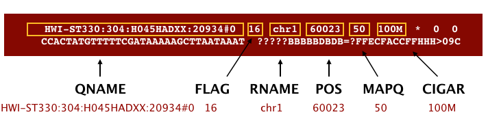
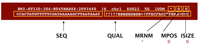
The file begins with a header, which is optional. The header is used to describe the source of data, reference sequence, method of alignment, etc., this will change depending on the aligner being used. Following the header is the alignment section. Each line that follows corresponds to alignment information for a single read. Each alignment line has 11 mandatory fields for essential mapping information and a variable number of other fields for aligner specific information. An example entry from a SAM file is displayed below with the different fields highlighted.
We will convert the SAM file to BAM format using the
samtools program with the view command and
tell this command that the input is in SAM format (-S) and
to output BAM format (-b):
OUTPUT
[samopen] SAM header is present: 1 sequences.Sort BAM file by coordinates
Next we sort the BAM file using the sort command from
samtools. -o tells the command where to write
the output.
BASH
$ samtools sort -o results/bam/SRR2584866.aligned.sorted.bam results/bam/SRR2584866.aligned.bam Our files are pretty small, so we will not see this output. If you run the workflow with larger files, you will see something like this:
OUTPUT
[bam_sort_core] merging from 2 files...SAM/BAM files can be sorted in multiple ways, e.g. by location of alignment on the chromosome, by read name, etc. It is important to be aware that different alignment tools will output differently sorted SAM/BAM, and different downstream tools require differently sorted alignment files as input.
You can use samtools to learn more about this bam file as well.
This will give you the following statistics about your sorted bam file:
OUTPUT
351169 + 0 in total (QC-passed reads + QC-failed reads)
0 + 0 secondary
1169 + 0 supplementary
0 + 0 duplicates
351103 + 0 mapped (99.98% : N/A)
350000 + 0 paired in sequencing
175000 + 0 read1
175000 + 0 read2
346688 + 0 properly paired (99.05% : N/A)
349876 + 0 with itself and mate mapped
58 + 0 singletons (0.02% : N/A)
0 + 0 with mate mapped to a different chr
0 + 0 with mate mapped to a different chr (mapQ>=5)
Variant calling
A variant call is a conclusion that there is a nucleotide difference
vs. some reference at a given position in an individual genome or
transcriptome, often referred to as a Single Nucleotide Variant (SNV).
The call is usually accompanied by an estimate of variant frequency and
some measure of confidence. Similar to other steps in this workflow,
there are a number of tools available for variant calling. In this
workshop we will be using bcftools, but there are a few
things we need to do before actually calling the variants.
Step 1: Calculate the read coverage of positions in the genome
Do the first pass on variant calling by counting read coverage with
bcftools.
We will use the command mpileup. The flag -O b
tells bcftools to generate a bcf format output file, -o
specifies where to write the output file, and -f flags the
path to the reference genome:
BASH
$ bcftools mpileup -O b -o results/bcf/SRR2584866_raw.bcf \
-f data/ref_genome/ecoli_rel606.fasta results/bam/SRR2584866.aligned.sorted.bam
OUTPUT
[mpileup] 1 samples in 1 input filesWe have now generated a file with coverage information for every base.
Step 2: Detect the single nucleotide variants (SNVs)
Identify SNVs using bcftools call. We have to specify
ploidy with the flag --ploidy, which is one for the haploid
E. coli. -m allows for multiallelic and
rare-variant calling, -v tells the program to output
variant sites only (not every site in the genome), and -o
specifies where to write the output file:
Step 3: Filter and report the SNV variants in variant calling format (VCF)
Filter the SNVs for the final output in VCF format, using
vcfutils.pl:
BASH
$ vcfutils.pl varFilter results/vcf/SRR2584866_variants.vcf > results/vcf/SRR2584866_final_variants.vcfFiltering
The vcfutils.pl varFilter call filters out variants that
do not meet minimum quality default criteria, which can be changed
through its options. Using bcftools we can verify that the
quality of the variant call set has improved after this filtering step
by calculating the ratio of transitions(TS)
to transversions
(TV) ratio (TS/TV), where transitions should be more likely to occur
than transversions:
BASH
$ bcftools stats results/vcf/SRR2584866_variants.vcf | grep TSTV
# TSTV, transitions/transversions:
# TSTV	[2]id	[3]ts	[4]tv	[5]ts/tv	[6]ts (1st ALT)	[7]tv (1st ALT)	[8]ts/tv (1st ALT)
TSTV	0	628	58	10.83	628	58	10.83
$ bcftools stats results/vcf/SRR2584866_final_variants.vcf | grep TSTV
# TSTV, transitions/transversions:
# TSTV	[2]id	[3]ts	[4]tv	[5]ts/tv	[6]ts (1st ALT)	[7]tv (1st ALT)	[8]ts/tv (1st ALT)
TSTV	0	621	54	11.50	621	54	11.50
Explore the VCF format:
You will see the header (which describes the format), the time and date the file was created, the version of bcftools that was used, the command line parameters used, and some additional information:
OUTPUT
##fileformat=VCFv4.2
##FILTER=<ID=PASS,Description="All filters passed">
##bcftoolsVersion=1.8+htslib-1.8
##bcftoolsCommand=mpileup -O b -o results/bcf/SRR2584866_raw.bcf -f data/ref_genome/ecoli_rel606.fasta results/bam/SRR2584866.aligned.sorted.bam
##reference=file://data/ref_genome/ecoli_rel606.fasta
##contig=<ID=CP000819.1,length=4629812>
##ALT=<ID=*,Description="Represents allele(s) other than observed.">
##INFO=<ID=INDEL,Number=0,Type=Flag,Description="Indicates that the variant is an INDEL.">
##INFO=<ID=IDV,Number=1,Type=Integer,Description="Maximum number of reads supporting an indel">
##INFO=<ID=IMF,Number=1,Type=Float,Description="Maximum fraction of reads supporting an indel">
##INFO=<ID=DP,Number=1,Type=Integer,Description="Raw read depth">
##INFO=<ID=VDB,Number=1,Type=Float,Description="Variant Distance Bias for filtering splice-site artefacts in RNA-seq data (bigger is better)",Version=
##INFO=<ID=RPB,Number=1,Type=Float,Description="Mann-Whitney U test of Read Position Bias (bigger is better)">
##INFO=<ID=MQB,Number=1,Type=Float,Description="Mann-Whitney U test of Mapping Quality Bias (bigger is better)">
##INFO=<ID=BQB,Number=1,Type=Float,Description="Mann-Whitney U test of Base Quality Bias (bigger is better)">
##INFO=<ID=MQSB,Number=1,Type=Float,Description="Mann-Whitney U test of Mapping Quality vs Strand Bias (bigger is better)">
##INFO=<ID=SGB,Number=1,Type=Float,Description="Segregation based metric.">
##INFO=<ID=MQ0F,Number=1,Type=Float,Description="Fraction of MQ0 reads (smaller is better)">
##FORMAT=<ID=PL,Number=G,Type=Integer,Description="List of Phred-scaled genotype likelihoods">
##FORMAT=<ID=GT,Number=1,Type=String,Description="Genotype">
##INFO=<ID=ICB,Number=1,Type=Float,Description="Inbreeding Coefficient Binomial test (bigger is better)">
##INFO=<ID=HOB,Number=1,Type=Float,Description="Bias in the number of HOMs number (smaller is better)">
##INFO=<ID=AC,Number=A,Type=Integer,Description="Allele count in genotypes for each ALT allele, in the same order as listed">
##INFO=<ID=AN,Number=1,Type=Integer,Description="Total number of alleles in called genotypes">
##INFO=<ID=DP4,Number=4,Type=Integer,Description="Number of high-quality ref-forward , ref-reverse, alt-forward and alt-reverse bases">
##INFO=<ID=MQ,Number=1,Type=Integer,Description="Average mapping quality">
##bcftools_callVersion=1.8+htslib-1.8
##bcftools_callCommand=call --ploidy 1 -m -v -o results/bcf/SRR2584866_variants.vcf results/bcf/SRR2584866_raw.bcf; Date=Tue Oct  9 18:48:10 2018
Followed by information on each of the variations observed:
OUTPUT
#CHROM  POS     ID      REF     ALT     QUAL    FILTER  INFO    FORMAT  results/bam/SRR2584866.aligned.sorted.bam
CP000819.1      1521    .       C       T       207     .       DP=9;VDB=0.993024;SGB=-0.662043;MQSB=0.974597;MQ0F=0;AC=1;AN=1;DP4=0,0,4,5;MQ=60
CP000819.1      1612    .       A       G       225     .       DP=13;VDB=0.52194;SGB=-0.676189;MQSB=0.950952;MQ0F=0;AC=1;AN=1;DP4=0,0,6,5;MQ=60
CP000819.1      9092    .       A       G       225     .       DP=14;VDB=0.717543;SGB=-0.670168;MQSB=0.916482;MQ0F=0;AC=1;AN=1;DP4=0,0,7,3;MQ=60
CP000819.1      9972    .       T       G       214     .       DP=10;VDB=0.022095;SGB=-0.670168;MQSB=1;MQ0F=0;AC=1;AN=1;DP4=0,0,2,8;MQ=60      GT:PL
CP000819.1      10563   .       G       A       225     .       DP=11;VDB=0.958658;SGB=-0.670168;MQSB=0.952347;MQ0F=0;AC=1;AN=1;DP4=0,0,5,5;MQ=60
CP000819.1      22257   .       C       T       127     .       DP=5;VDB=0.0765947;SGB=-0.590765;MQSB=1;MQ0F=0;AC=1;AN=1;DP4=0,0,2,3;MQ=60      GT:PL
CP000819.1      38971   .       A       G       225     .       DP=14;VDB=0.872139;SGB=-0.680642;MQSB=1;MQ0F=0;AC=1;AN=1;DP4=0,0,4,8;MQ=60      GT:PL
CP000819.1      42306   .       A       G       225     .       DP=15;VDB=0.969686;SGB=-0.686358;MQSB=1;MQ0F=0;AC=1;AN=1;DP4=0,0,5,9;MQ=60      GT:PL
CP000819.1      45277   .       A       G       225     .       DP=15;VDB=0.470998;SGB=-0.680642;MQSB=0.95494;MQ0F=0;AC=1;AN=1;DP4=0,0,7,5;MQ=60
CP000819.1      56613   .       C       G       183     .       DP=12;VDB=0.879703;SGB=-0.676189;MQSB=1;MQ0F=0;AC=1;AN=1;DP4=0,0,8,3;MQ=60      GT:PL
CP000819.1      62118   .       A       G       225     .       DP=19;VDB=0.414981;SGB=-0.691153;MQSB=0.906029;MQ0F=0;AC=1;AN=1;DP4=0,0,8,10;MQ=59
CP000819.1      64042   .       G       A       225     .       DP=18;VDB=0.451328;SGB=-0.689466;MQSB=1;MQ0F=0;AC=1;AN=1;DP4=0,0,7,9;MQ=60      GT:PL
This is a lot of information, so let’s take some time to make sure we understand our output.
The first few columns represent the information we have about a predicted variation.
| column | info |
|---|---|
| CHROM | contig location where the variation occurs |
| POS | position within the contig where the variation occurs |
| ID | a . until we add annotation information |
| REF | reference genotype (forward strand) |
| ALT | sample genotype (forward strand) |
| QUAL | Phred-scaled probability that the observed variant exists at this site (higher is better) |
| FILTER | a . if no quality filters have been applied, PASS if a
filter is passed, or the name of the filters this variant failed |
In an ideal world, the information in the QUAL column
would be all we needed to filter out bad variant calls. However, in
reality we need to filter on multiple other metrics.
The last two columns contain the genotypes and can be tricky to decode.
| column | info |
|---|---|
| FORMAT | lists in order the metrics presented in the final column |
| results | lists the values associated with those metrics in order |
For our file, the metrics presented are GT:PL:GQ.
| metric | definition |
|---|---|
| AD, DP | the depth per allele by sample and coverage |
| GT | the genotype for the sample at this loci. For a diploid organism, the GT field indicates the two alleles carried by the sample, encoded by a 0 for the REF allele, 1 for the first ALT allele, 2 for the second ALT allele, etc. A 0/0 means homozygous reference, 0/1 is heterozygous, and 1/1 is homozygous for the alternate allele. |
| PL | the likelihoods of the given genotypes |
| GQ | the Phred-scaled confidence for the genotype |
The Broad Institute’s VCF guide is an excellent place to learn more about the VCF file format.
Exercise
Use the grep and wc commands you have
learned to assess how many variants are in the vcf file.
Assess the alignment (visualization) - optional step
It is often instructive to look at your data in a genome browser. Visualization will allow you to get a “feel” for the data, as well as detecting abnormalities and problems. Also, exploring the data in such a way may give you ideas for further analyses. As such, visualization tools are useful for exploratory analysis. In this lesson we will describe two different tools for visualization: a light-weight command-line based one and the Broad Institute’s Integrative Genomics Viewer (IGV) which requires software installation and transfer of files.
In order for us to visualize the alignment files, we will need to
index the BAM file using samtools:
Viewing with tview
Samtools implements a very
simple text alignment viewer based on the GNU ncurses
library, called tview. This alignment viewer works with
short indels and shows MAQ
consensus. It uses different colors to display mapping quality or base
quality, subjected to users’ choice. Samtools viewer is known to work
with a 130 GB alignment swiftly. Due to its text interface, displaying
alignments over network is also very fast.
In order to visualize our mapped reads, we use tview,
giving it the sorted bam file and the reference file:
OUTPUT
1         11        21        31        41        51        61        71        81        91        101       111       121
AGCTTTTCATTCTGACTGCAACGGGCAATATGTCTCTGTGTGGATTAAAAAAAGAGTGTCTGATAGCAGCTTCTGAACTGGTTACCTGCCGTGAGTAAATTAAAATTTTATTGACTTAGGTCACTAAATAC
..................................................................................................................................
,,,,,,,,,,,,,,,,,,,,,,,,,,,,,,,,,,,, ..................N................. ,,,,,,,,,,,,,,,,,,,,,,,,,,,,,,,,........................
,,,,,,,,,,,,,,,,,,,,,,,,,,,,,,,,,,, ..................N................. ,,,,,,,,,,,,,,,,,,,,,,,,,,,.............................
...................................,g,,,,,,,,,,,,,,,,,,,,,,,,,,,,,,,,,  ....................................   ................
,,,,,,,,,,,,,,,,,,,,,,,,,,,,,,,,,,,....................................   ....................................      ,,,,,,,,,,
,,,,,,,,,,,,,,,,,,,,,,,,,,,,,,,,,,,,  ....................................  ,,a,,,,,,,,,,,,,,,,,,,,,,,,,,,,,     .......
,,,,,,,,,,,,,,,,,,,,,,,,,,,,,,, .............................  ,,,,,,,,,,,,,,,,,g,,,,,    ,,,,,,,,,,,,,,,,,,,,,,,,,,,,
,,,,,,,,,,,,,,,,,,,,,,,,,,,,,,,,,,,  ...........................T.......   ,,,,,,,,,,,,,,,,,,,,,,,c,          ......
......................... ................................   ,g,,,,,,,,,,,,,,,,,,,      ...........................
,,,,,,,,,,,,,,,,,,,,, ,,,,,,,,,,,,,,,,,,,,,,,,,,,,,,, ,,,,,,,,,,,,,,,,,,,,,,,,,,,       ..........................
,,,,,,,,,,,,,,,,,,,,,,,,,,,,,,,,,,,   ................................T..  ..............................   ,,,,,,
...........................       ,,,,,,g,,,,,,,,,,,,,,,,,   ....................................         ,,,,,,
,,,,,,,,,,,,,,,,,,,,,,,,,, ....................................  ...................................        ....
....................................  ........................  ,,,,,,,,,,,,,,,,,,,,,,,,,,,,,,,,,,,,      ....
,,,,,,,,,,,,,,,,,,,,,,,,,,,,,,,,,,,,   ,,,,,,,,,,,,,,,,,,,,,,,,,,,,,,,,,,,,  ,,,,,,,,,,,,,,,,,,,,,,,,,,,,,,,,,
........................            .................................. .............................     ....
,,,,,,,,,,,,,,,,,,,,,,,,,,,,,,,,,,,,   ....................................        ..........................
...............................       ,,,,,,,,,,,,,,,,,,,,,,,,,,,,,,,, ....................................
...................................  ,,,,,,,,,,,,,,,,,,,,,,,,,,,,,,,,  ,,,,,,,,,,,,,,,,,,,,,,,,,,,,,,,,,,,
,,,,,,,,,,,,,,,,,,,,,,,,,,,,,,,,,,,, ,,,,,,,,,,,,,,,,,,,,,,,,,,,,,,,,,,  ..................................
.................................... ,,,,,,,,,,,,,,,,,,a,,,,,,,,,,,,,,,,,        ,,,,,,,,,,,,,,,,,,,,,,,,,
,,,,,,,,,,,,,,,,,,,,,,,,,,,,,,,,,,,  ............................ ,,,,,,,,,,,,,,,,,,,,,,,,,,,,,,,,,,,,
The first line of output shows the genome coordinates in our
reference genome. The second line shows the reference genome sequence.
The third line shows the consensus sequence determined from the sequence
reads. A . indicates a match to the reference sequence, so
we can see that the consensus from our sample matches the reference in
most locations. That is good! If that was not the case, we should
probably reconsider our choice of reference.
Below the horizontal line, we can see all of the reads in our sample
aligned with the reference genome. Only positions where the called base
differs from the reference are shown. You can use the arrow keys on your
keyboard to scroll or type ? for a help menu. To navigate
to a specific position, type g. A dialogue box will appear.
In this box, type the name of the “chromosome” followed by a colon and
the position of the variant you would like to view (e.g. for this
sample, type CP000819.1:50 to view the 50th base. Type
Ctrl^C or q to exit tview.
Exercise
Visualize the alignment of the reads for our SRR2584866
sample. What variant is present at position 4377265? What is the
canonical nucleotide in that position?
BASH
$ samtools tview ~/dc_workshop/results/bam/SRR2584866.aligned.sorted.bam ~/dc_workshop/data/ref_genome/ecoli_rel606.fastaThen type g. In the dialogue box, type
CP000819.1:4377265. G is the variant.
A is canonical. This variant possibly changes the phenotype
of this sample to hypermutable. It occurs in the gene mutL,
which controls DNA mismatch repair.
Viewing with IGV
IGV is a stand-alone browser, which has the advantage of being installed locally and providing fast access. Web-based genome browsers, like Ensembl or the UCSC browser, are slower, but provide more functionality. They not only allow for more polished and flexible visualization, but also provide easy access to a wealth of annotations and external data sources. This makes it straightforward to relate your data with information about repeat regions, known genes, epigenetic features or areas of cross-species conservation, to name just a few.
In order to use IGV, we will need to transfer some files to our local
machine. We know how to do this with scp. Open a new tab in
your terminal window and create a new folder. We will put this folder on
our Desktop for demonstration purposes, but in general you should avoid
proliferating folders and files on your Desktop and instead organize
files within a directory structure like we have been using in our
dc_workshop directory.
Now we will transfer our files to that new directory. Remember to
replace the text between the @ and the : with
your AWS instance number. The commands to scp always go in
the terminal window that is connected to your local computer (not your
AWS instance).
BASH
$ scp dcuser@ec2-34-203-203-131.compute-1.amazonaws.com:~/dc_workshop/results/bam/SRR2584866.aligned.sorted.bam ~/Desktop/files_for_igv
$ scp dcuser@ec2-34-203-203-131.compute-1.amazonaws.com:~/dc_workshop/results/bam/SRR2584866.aligned.sorted.bam.bai ~/Desktop/files_for_igv
$ scp dcuser@ec2-34-203-203-131.compute-1.amazonaws.com:~/dc_workshop/data/ref_genome/ecoli_rel606.fasta ~/Desktop/files_for_igv
$ scp dcuser@ec2-34-203-203-131.compute-1.amazonaws.com:~/dc_workshop/results/vcf/SRR2584866_final_variants.vcf ~/Desktop/files_for_igv
You will need to type the password for your AWS instance each time
you call scp.
Next, we need to open the IGV software. If you have not done so
already, you can download IGV from the Broad
Institute’s software page, double-click the .zip file
to unzip it, and then drag the program into your Applications
folder.
- Open IGV.
- Load our reference genome file (
ecoli_rel606.fasta) into IGV using the “Load Genomes from File…” option under the “Genomes” pull-down menu. - Load our BAM file (
SRR2584866.aligned.sorted.bam) using the “Load from File…” option under the “File” pull-down menu. - Do the same with our VCF file
(
SRR2584866_final_variants.vcf).
Your IGV browser should look like the screenshot below:
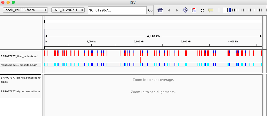
There should be two tracks: one coresponding to our BAM file and the other for our VCF file.
In the VCF track, each bar across the top of the plot shows the allele fraction for a single locus. The second bar shows the genotypes for each locus in each sample. We only have one sample called here, so we only see a single line. Dark blue = heterozygous, Cyan = homozygous variant, Grey = reference. Filtered entries are transparent.
Zoom in to inspect variants you see in your filtered VCF file to become more familiar with IGV. See how quality information corresponds to alignment information at those loci. Use this website and the links therein to understand how IGV colors the alignments.
Now that we have run through our workflow for a single sample, we want to repeat this workflow for our other five samples. However, we do not want to type each of these individual steps again five more times. That would be very time consuming and error-prone, and would become impossible as we gathered more and more samples. Luckily, we already know the tools we need to use to automate this workflow and run it on as many files as we want using a single line of code. Those tools are: wildcards, for loops, and bash scripts. We will use all three in the next lesson.
Installing software
It is worth noting that all of the software we are using for this workshop has been pre-installed on our remote computer. This saves us a lot of time - installing software can be a time-consuming and frustrating task - however, this does mean that you will not be able to walk out the door and start doing these analyses on your own computer. You will need to install the software first. Look at the setup instructions for more information on installing these software packages.
BWA alignment options
BWA consists of three algorithms: BWA-backtrack, BWA-SW and BWA-MEM. The first algorithm is designed for Illumina sequence reads up to 100bp, while the other two are for sequences ranging from 70bp to 1Mbp. BWA-MEM and BWA-SW share similar features such as long-read support and split alignment, but BWA-MEM, which is the latest, is generally recommended for high-quality queries as it is faster and more accurate.
Key Points
- Bioinformatic command line tools are collections of commands that can be used to carry out bioinformatic analyses.
- To use most powerful bioinformatic tools, you will need to use the command line.
- There are many different file formats for storing genomics data. It is important to understand what type of information is contained in each file, and how it was derived.
Content from Automating a Variant Calling Workflow
Last updated on 2024-07-08 | Edit this page
Overview
Questions
- How can I make my workflow more efficient and less error-prone?
Objectives
- Write a shell script with multiple variables.
- Incorporate a
forloop into a shell script.
What is a shell script?
You wrote a simple shell script in a previous lesson that we used to extract bad reads from our FASTQ files and put them into a new file.
Here is the script you wrote:
That script was only two lines long, but shell scripts can be much more complicated than that and can be used to perform a large number of operations on one or many files. This saves you the effort of having to type each of those commands over for each of your data files and makes your work less error-prone and more reproducible. For example, the variant calling workflow we just carried out had about eight steps where we had to type a command into our terminal. Most of these commands were pretty long. If we wanted to do this for all six of our data files, that would be forty-eight steps. If we had 50 samples (a more realistic number), it would be 400 steps! You can see why we want to automate this.
We have also used for loops in previous lessons to
iterate one or two commands over multiple input files. In these
for loops, the filename was defined as a variable in the
for statement, which enabled you to run the loop on
multiple files. We will be using variable assignments like this in our
new shell scripts.
Here is the for loop you wrote for unzipping
.zip files:
And here is the one you wrote for running Trimmomatic on all of our
.fastq sample files:
BASH
$ for infile in *_1.fastq.gz
> do
>   base=$(basename ${infile} _1.fastq.gz)
>   trimmomatic PE ${infile} ${base}_2.fastq.gz \
>                ${base}_1.trim.fastq.gz ${base}_1un.trim.fastq.gz \
>                ${base}_2.trim.fastq.gz ${base}_2un.trim.fastq.gz \
>                SLIDINGWINDOW:4:20 MINLEN:25 ILLUMINACLIP:NexteraPE-PE.fa:2:40:15
> done
Notice that in this for loop, we used two variables,
infile, which was defined in the for
statement, and base, which was created from the filename
during each iteration of the loop.
Creating variables
Within the Bash shell you can create variables at any time (as we did above, and during the ‘for’ loop lesson). Assign any name and the value using the assignment operator: ‘=’. You can check the current definition of your variable by typing into your script: echo $variable_name.
In this lesson, we will use two shell scripts to automate the variant
calling analysis: one for FastQC analysis (including creating our
summary file), and a second for the remaining variant calling. To write
a script to run our FastQC analysis, we will take each of the commands
we entered to run FastQC and process the output files and put them into
a single file with a .sh extension. The .sh is
not essential, but serves as a reminder to ourselves and to the computer
that this is a shell script.
Analyzing quality with FastQC
We will use the command touch to create a new file where
we will write our shell script. We will create this script in a new
directory called scripts/. Previously, we used
nano to create and open a new file. The command
touch allows us to create a new file without opening that
file.
OUTPUT
read_qc.shWe now have an empty file called read_qc.sh in our
scripts/ directory. We will now open this file in
nano and start building our script.
Enter the following pieces of code into your shell script (not into your terminal prompt).
Our first line will ensure that our script will exit if an error
occurs, and is a good idea to include at the beginning of your scripts.
The second line will move us into the untrimmed_fastq/
directory when we run our script.
OUTPUT
set -e
cd ~/dc_workshop/data/untrimmed_fastq/
These next two lines will give us a status message to tell us that we
are currently running FastQC, then will run FastQC on all of the files
in our current directory with a .fastq extension.
OUTPUT
echo "Running FastQC ..."
fastqc *.fastq*
Our next line will create a new directory to hold our FastQC output
files. Here we are using the -p option for
mkdir again. It is a good idea to use this option in your
shell scripts to avoid running into errors if you do not have the
directory structure you think you do.
OUTPUT
mkdir -p ~/dc_workshop/results/fastqc_untrimmed_readsOur next three lines first give us a status message to tell us we are
saving the results from FastQC, then moves all of the files with a
.zip or a .html extension to the directory we
just created for storing our FastQC results.
OUTPUT
echo "Saving FastQC results..."
mv *.zip ~/dc_workshop/results/fastqc_untrimmed_reads/
mv *.html ~/dc_workshop/results/fastqc_untrimmed_reads/
The next line moves us to the results directory where we have stored our output.
OUTPUT
cd ~/dc_workshop/results/fastqc_untrimmed_reads/The next five lines should look very familiar. First we give
ourselves a status message to tell us that we are unzipping our ZIP
files. Then we run our for loop to unzip all of the .zip
files in this directory.
OUTPUT
echo "Unzipping..."
for filename in *.zip
    do
    unzip $filename
    done
Next we concatenate all of our summary files into a single output file, with a status message to remind ourselves that this is what we are doing.
OUTPUT
echo "Saving summary..."
mkdir -p ~/dc_workshops/docs
cat */summary.txt > ~/dc_workshop/docs/fastqc_summaries.txt
Using echo statements
We have used echo statements to add progress statements
to our script. Our script will print these statements as it is running
and therefore we will be able to see how far our script has
progressed.
Your full shell script should now look like this:
OUTPUT
set -e
cd ~/dc_workshop/data/untrimmed_fastq/

echo "Running FastQC ..."
fastqc *.fastq*

mkdir -p ~/dc_workshop/results/fastqc_untrimmed_reads

echo "Saving FastQC results..."
mv *.zip ~/dc_workshop/results/fastqc_untrimmed_reads/
mv *.html ~/dc_workshop/results/fastqc_untrimmed_reads/

cd ~/dc_workshop/results/fastqc_untrimmed_reads/

echo "Unzipping..."
for filename in *.zip
    do
    unzip $filename
    done

echo "Saving summary..."
cat */summary.txt > ~/dc_workshop/docs/fastqc_summaries.txt
Save your file and exit nano. We can now run our
script:
OUTPUT
Running FastQC ...
Started analysis of SRR2584866.fastq
Approx 5% complete for SRR2584866.fastq
Approx 10% complete for SRR2584866.fastq
Approx 15% complete for SRR2584866.fastq
Approx 20% complete for SRR2584866.fastq
Approx 25% complete for SRR2584866.fastq
.
.
.
For each of your sample files, FastQC will ask if you want to replace
the existing version with a new version. This is because we have already
run FastQC on this samples files and generated all of the outputs. We
are now doing this again using our scripts. Go ahead and select
A each time this message appears. It will appear once per
sample file (six times total).
OUTPUT
replace SRR2584866_fastqc/Icons/fastqc_icon.png? [y]es, [n]o, [A]ll, [N]one, [r]ename:Automating the rest of our variant calling workflow
We can extend these principles to the entire variant calling
workflow. To do this, we will take all of the individual commands that
we wrote before, put them into a single file, add variables so that the
script knows to iterate through our input files and write to the
appropriate output files. This is very similar to what we did with our
read_qc.sh script, but will be a bit more complex.
Download the script from here. Download to
~/dc_workshop/scripts.
Our variant calling workflow has the following steps:
- Index the reference genome for use by bwa and samtools.
- Align reads to reference genome.
- Convert the format of the alignment to sorted BAM, with some intermediate steps.
- Calculate the read coverage of positions in the genome.
- Detect the single nucleotide variants (SNVs).
- Filter and report the SNVs in VCF (variant calling format).
Let’s go through this script together:
The script should look like this:
OUTPUT
set -e
cd ~/dc_workshop/results

genome=~/dc_workshop/data/ref_genome/ecoli_rel606.fasta

bwa index $genome

mkdir -p sam bam bcf vcf

for fq1 in ~/dc_workshop/data/trimmed_fastq_small/*_1.trim.sub.fastq
    do
    echo "working with file $fq1"

    base=$(basename $fq1 _1.trim.sub.fastq)
    echo "base name is $base"

    fq1=~/dc_workshop/data/trimmed_fastq_small/${base}_1.trim.sub.fastq
    fq2=~/dc_workshop/data/trimmed_fastq_small/${base}_2.trim.sub.fastq
    sam=~/dc_workshop/results/sam/${base}.aligned.sam
    bam=~/dc_workshop/results/bam/${base}.aligned.bam
    sorted_bam=~/dc_workshop/results/bam/${base}.aligned.sorted.bam
    raw_bcf=~/dc_workshop/results/bcf/${base}_raw.bcf
    variants=~/dc_workshop/results/vcf/${base}_variants.vcf
    final_variants=~/dc_workshop/results/vcf/${base}_final_variants.vcf

    bwa mem $genome $fq1 $fq2 > $sam
    samtools view -S -b $sam > $bam
    samtools sort -o $sorted_bam $bam
    samtools index $sorted_bam
    bcftools mpileup -O b -o $raw_bcf -f $genome $sorted_bam
    bcftools call --ploidy 1 -m -v -o $variants $raw_bcf
    vcfutils.pl varFilter $variants > $final_variants

    done
Now, we will go through each line in the script before running it.
First, notice that we change our working directory so that we can create new results subdirectories in the right location.
OUTPUT
cd ~/dc_workshop/resultsNext we tell our script where to find the reference genome by
assigning the genome variable to the path to our reference
genome:
OUTPUT
genome=~/dc_workshop/data/ref_genome/ecoli_rel606.fastaNext we index our reference genome for BWA:
OUTPUT
bwa index $genomeAnd create the directory structure to store our results in:
OUTPUT
mkdir -p sam bam bcf vcfThen, we use a loop to run the variant calling workflow on each of
our FASTQ files. The full list of commands within the loop will be
executed once for each of the FASTQ files in the
data/trimmed_fastq_small/ directory. We will include a few
echo statements to give us status updates on our
progress.
The first thing we do is assign the name of the FASTQ file we are
currently working with to a variable called fq1 and tell
the script to echo the filename back to us so we can check
which file we are on.
BASH
for fq1 in ~/dc_workshop/data/trimmed_fastq_small/*_1.trim.sub.fastq
    do
    echo "working with file $fq1"
We then extract the base name of the file (excluding the path and
.fastq extension) and assign it to a new variable called
base.
We can use the base variable to access both the
base_1.fastq and base_2.fastq input files, and
create variables to store the names of our output files. This makes the
script easier to read because we do not need to type out the full name
of each of the files: instead, we use the base variable,
but add a different extension (e.g. .sam,
.bam) for each file produced by our workflow.
BASH
    #input fastq files
    fq1=~/dc_workshop/data/trimmed_fastq_small/${base}_1.trim.sub.fastq
    fq2=~/dc_workshop/data/trimmed_fastq_small/${base}_2.trim.sub.fastq

    # output files
    sam=~/dc_workshop/results/sam/${base}.aligned.sam
    bam=~/dc_workshop/results/bam/${base}.aligned.bam
    sorted_bam=~/dc_workshop/results/bam/${base}.aligned.sorted.bam
    raw_bcf=~/dc_workshop/results/bcf/${base}_raw.bcf
    variants=~/dc_workshop/results/bcf/${base}_variants.vcf
    final_variants=~/dc_workshop/results/vcf/${base}_final_variants.vcf
And finally, the actual workflow steps:
- align the reads to the reference genome and output a
.samfile:
OUTPUT
bwa mem $genome $fq1 $fq2 > $sam- convert the SAM file to BAM format:
OUTPUT
samtools view -S -b $sam > $bam- sort the BAM file:
OUTPUT
samtools sort -o $sorted_bam $bam - index the BAM file for display purposes:
OUTPUT
samtools index $sorted_bam- calculate the read coverage of positions in the genome:
OUTPUT
bcftools mpileup -O b -o $raw_bcf -f $genome $sorted_bam - call SNVs with bcftools:
OUTPUT
bcftools call --ploidy 1 -m -v -o $variants $raw_bcf - filter and report the SNVs in variant calling format (VCF):
OUTPUT
vcfutils.pl varFilter $variants > $final_variantsExercise
It is a good idea to add comments to your code so that you (or a
collaborator) can make sense of what you did later. Look through your
existing script. Discuss with a neighbor where you should add comments.
Add comments (anything following a # character will be
interpreted as a comment, bash will not try to run these comments as
code).
Now we can run our script:
Exercise
The samples we just performed variant calling on are part of the long-term evolution experiment introduced at the beginning of our variant calling workflow. From the metadata table, we know that SRR2589044 was from generation 5000, SRR2584863 was from generation 15000, and SRR2584866 was from generation 50000. How did the number of mutations per sample change over time? Examine the metadata table. What is one reason the number of mutations may have changed the way they did?
Hint: You can find a copy of the output files for the subsampled
trimmed FASTQ file variant calling in the
~/.solutions/wrangling-solutions/variant_calling_auto/
directory.
BASH
$ for infile in ~/dc_workshop/results/vcf/*_final_variants.vcf
> do
>     echo ${infile}
>     grep -v "#" ${infile} | wc -l
> done
For SRR2589044 from generation 5000 there were 10 mutations, for SRR2584863 from generation 15000 there were 25 mutations, and SRR2584866 from generation 50000 there were 766 mutations. In the last generation, a hypermutable phenotype had evolved, causing this strain to have more mutations.
Bonus exercise
If you have time after completing the previous exercise, use
run_variant_calling.sh to run the variant calling pipeline
on the full-sized trimmed FASTQ files. You should have a copy of these
already in ~/dc_workshop/data/trimmed_fastq, but if you do
not, there is a copy in
~/.solutions/wrangling-solutions/trimmed_fastq. Does the
number of variants change per sample?
Key Points
- We can combine multiple commands into a shell script to automate a workflow.
- Use
echostatements within your scripts to get an automated progress update.