Starting with Data
Last updated on 2024-07-02 | Edit this page
Estimated time: 80 minutes
The two main goals for this lessons are:
- To make sure that learners are comfortable with working with data frames, and can use the bracket notation to select slices/columns.
- To expose learners to factors. Their behavior is not necessarily intuitive, and so it is important that they are guided through it the first time they are exposed to it. The content of the lesson should be enough for learners to avoid common mistakes with them.
Overview
Questions
- What is a data.frame?
- How can I read a complete csv file into R?
- How can I get basic summary information about my dataset?
- How can I change the way R treats strings in my dataset?
- Why would I want strings to be treated differently?
- How are dates represented in R and how can I change the format?
Objectives
- Describe what a data frame is.
- Load external data from a .csv file into a data frame.
- Summarize the contents of a data frame.
- Subset values from data frames.
- Describe the difference between a factor and a string.
- Convert between strings and factors.
- Reorder and rename factors.
- Change how character strings are handled in a data frame.
- Examine and change date formats.
What are data frames?
Data frames are the de facto data structure for tabular data
in R, and what we use for data processing, statistics, and
plotting.
A data frame is the representation of data in the format of a table where the columns are vectors that all have the same length. Data frames are analogous to the more familiar spreadsheet in programs such as Excel, with one key difference. Because columns are vectors, each column must contain a single type of data (e.g., characters, integers, factors). For example, here is a figure depicting a data frame comprising a numeric, a character, and a logical vector.

Data frames can be created by hand, but most commonly they are
generated by the functions read_csv() or
read_table(); in other words, when importing spreadsheets
from your hard drive (or the web). We will now demonstrate how to import
tabular data using read_csv().
Presentation of the SAFI Data
SAFI (Studying African Farmer-Led Irrigation) is a study looking at farming and irrigation methods in Tanzania and Mozambique. The survey data was collected through interviews conducted between November 2016 and June 2017. For this lesson, we will be using a subset of the available data. For information about the full teaching dataset used in other lessons in this workshop, see the dataset description.
We will be using a subset of the cleaned version of the dataset that
was produced through cleaning in OpenRefine
(data/SAFI_clean.csv). In this dataset, the missing data is
encoded as “NULL”, each row holds information for a single interview
respondent, and the columns represent:
| column_name | description |
|---|---|
| key_id | Added to provide a unique Id for each observation. (The InstanceID field does this as well but it is not as convenient to use) |
| village | Village name |
| interview_date | Date of interview |
| no_membrs | How many members in the household? |
| years_liv | How many years have you been living in this village or neighboring village? |
| respondent_wall_type | What type of walls does their house have (from list) |
| rooms | How many rooms in the main house are used for sleeping? |
| memb_assoc | Are you a member of an irrigation association? |
| affect_conflicts | Have you been affected by conflicts with other irrigators in the area? |
| liv_count | Number of livestock owned. |
| items_owned | Which of the following items are owned by the household? (list) |
| no_meals | How many meals do people in your household normally eat in a day? |
| months_lack_food | Indicate which months, In the last 12 months have you faced a situation when you did not have enough food to feed the household? |
| instanceID | Unique identifier for the form data submission |
Importing data
You are going to load the data in R’s memory using the function
read_csv() from the readr
package, which is part of the tidyverse;
learn more about the tidyverse collection
of packages here.
readr gets installed as part as the
tidyverse installation. When you load the
tidyverse
(library(tidyverse)), the core packages (the packages used
in most data analyses) get loaded, including
readr.
Before proceeding, however, this is a good opportunity to talk about
conflicts. Certain packages we load can end up introducing function
names that are already in use by pre-loaded R packages. For instance,
when we load the tidyverse package below, we will introduce two
conflicting functions: filter() and lag().
This happens because filter and lag are
already functions used by the stats package (already pre-loaded in R).
What will happen now is that if we, for example, call the
filter() function, R will use the
dplyr::filter() version and not the
stats::filter() one. This happens because, if conflicted,
by default R uses the function from the most recently loaded package.
Conflicted functions may cause you some trouble in the future, so it is
important that we are aware of them so that we can properly handle them,
if we want.
To do so, we just need the following functions from the conflicted package:
-
conflicted::conflict_scout(): Shows us any conflicted functions. -
conflict_prefer("function", "package_prefered"): Allows us to choose the default function we want from now on.
It is also important to know that we can, at any time, just call the
function directly from the package we want, such as
stats::filter().
Even with the use of an RStudio project, it can be difficult to learn
how to specify paths to file locations. Enter the here
package! The here package creates paths relative to the top-level
directory (your RStudio project). These relative paths work
regardless of where the associated source file lives inside
your project, like analysis projects with data and reports in different
subdirectories. This is an important contrast to using
setwd(), which depends on the way you order your files on
your computer.

Before we can use the read_csv() and here()
functions, we need to load the tidyverse and here packages.
Also, if you recall, the missing data is encoded as “NULL” in the
dataset. We’ll tell it to the function, so R will automatically convert
all the “NULL” entries in the dataset into NA.
R
library(tidyverse)
library(here)

interviews <- read_csv(
  here("data", "SAFI_clean.csv"),
  na = "NULL")
In the above code, we notice the here() function takes
folder and file names as inputs (e.g., "data",
"SAFI_clean.csv"), each enclosed in quotations
("") and separated by a comma. The here() will
accept as many names as are necessary to navigate to a particular file
(e.g.,
here("analysis", "data", "surveys", "clean", "SAFI_clean.csv)).
The here() function can accept the folder and file names
in an alternate format, using a slash (“/”) rather than commas to
separate the names. The two methods are equivalent, so that
here("data", "SAFI_clean.csv") and
here("data/SAFI_clean.csv") produce the same result. (The
slash is used on all operating systems; backslashes are not used.)
If you were to type in the code above, it is likely that the
read.csv() function would appear in the automatically
populated list of functions. This function is different from the
read_csv() function, as it is included in the “base”
packages that come pre-installed with R. Overall,
read.csv() behaves similar to read_csv(), with
a few notable differences. First, read.csv() coerces column
names with spaces and/or special characters to different names
(e.g. interview date becomes interview.date).
Second, read.csv() stores data as a
data.frame, where read_csv() stores data as a
different kind of data frame called a tibble. We prefer
tibbles because they have nice printing properties among other desirable
qualities. Read more about tibbles here.
The second statement in the code above creates a data frame but
doesn’t output any data because, as you might recall, assignments
(<-) don’t display anything. (Note, however, that
read_csv may show informational text about the data frame
that is created.) If we want to check that our data has been loaded, we
can see the contents of the data frame by typing its name:
interviews in the console.
R
interviews
## Try also
## view(interviews)
## head(interviews)
OUTPUT
# A tibble: 131 × 14
   key_ID village  interview_date      no_membrs years_liv respondent_wall_type
    <dbl> <chr>    <dttm>                  <dbl>     <dbl> <chr>
 1      1 God      2016-11-17 00:00:00         3         4 muddaub
 2      2 God      2016-11-17 00:00:00         7         9 muddaub
 3      3 God      2016-11-17 00:00:00        10        15 burntbricks
 4      4 God      2016-11-17 00:00:00         7         6 burntbricks
 5      5 God      2016-11-17 00:00:00         7        40 burntbricks
 6      6 God      2016-11-17 00:00:00         3         3 muddaub
 7      7 God      2016-11-17 00:00:00         6        38 muddaub
 8      8 Chirodzo 2016-11-16 00:00:00        12        70 burntbricks
 9      9 Chirodzo 2016-11-16 00:00:00         8         6 burntbricks
10     10 Chirodzo 2016-12-16 00:00:00        12        23 burntbricks
# ℹ 121 more rows
# ℹ 8 more variables: rooms <dbl>, memb_assoc <chr>, affect_conflicts <chr>,
#   liv_count <dbl>, items_owned <chr>, no_meals <dbl>, months_lack_food <chr>,
#   instanceID <chr>
Note
read_csv() assumes that fields are delimited by commas.
However, in several countries, the comma is used as a decimal separator
and the semicolon (;) is used as a field delimiter. If you want to read
in this type of files in R, you can use the read_csv2
function. It behaves exactly like read_csv but uses
different parameters for the decimal and the field separators. If you
are working with another format, they can be both specified by the user.
Check out the help for read_csv() by typing
?read_csv to learn more. There is also the
read_tsv() for tab-separated data files, and
read_delim() allows you to specify more details about the
structure of your file.
Note that read_csv() actually loads the data as a
tibble. A tibble is an extension of R data frames used by
the tidyverse. When the data is read using
read_csv(), it is stored in an object of class
tbl_df, tbl, and data.frame. You
can see the class of an object with
R
class(interviews)
OUTPUT
[1] "spec_tbl_df" "tbl_df" "tbl" "data.frame" As a tibble, the type of data included in each column is
listed in an abbreviated fashion below the column names. For instance,
here key_ID is a column of floating point numbers
(abbreviated <dbl> for the word ‘double’),
village is a column of characters
(<chr>) and the interview_date is a
column in the “date and time” format (<dttm>).
Inspecting data frames
When calling a tbl_df object (like
interviews here), there is already a lot of information
about our data frame being displayed such as the number of rows, the
number of columns, the names of the columns, and as we just saw the
class of data stored in each column. However, there are functions to
extract this information from data frames. Here is a non-exhaustive list
of some of these functions. Let’s try them out!
Size:
-
dim(interviews)- returns a vector with the number of rows as the first element, and the number of columns as the second element (the dimensions of the object) -
nrow(interviews)- returns the number of rows -
ncol(interviews)- returns the number of columns
Content:
-
head(interviews)- shows the first 6 rows -
tail(interviews)- shows the last 6 rows
Names:
-
names(interviews)- returns the column names (synonym ofcolnames()fordata.frameobjects)
Summary:
-
str(interviews)- structure of the object and information about the class, length and content of each column -
summary(interviews)- summary statistics for each column -
glimpse(interviews)- returns the number of columns and rows of the tibble, the names and class of each column, and previews as many values will fit on the screen. Unlike the other inspecting functions listed above,glimpse()is not a “base R” function so you need to have thedplyrortibblepackages loaded to be able to execute it.
Note: most of these functions are “generic.” They can be used on other types of objects besides data frames or tibbles.
Subsetting data frames
Our interviews data frame has rows and columns (it has 2
dimensions). In practice, we may not need the entire data frame; for
instance, we may only be interested in a subset of the observations (the
rows) or a particular set of variables (the columns). If we want to
access some specific data from it, we need to specify the “coordinates”
(i.e., indices) we want from it. Row numbers come first, followed by
column numbers.
Tip
Subsetting a tibble with [ always results
in a tibble. However, note this is not true in general for
data frames, so be careful! Different ways of specifying these
coordinates can lead to results with different classes. This is covered
in the Software Carpentry lesson R for
Reproducible Scientific Analysis.
R
## first element in the first column of the tibble
interviews[1, 1]
OUTPUT
# A tibble: 1 × 1
  key_ID
   <dbl>
1      1
R
## first element in the 6th column of the tibble
interviews[1, 6]
OUTPUT
# A tibble: 1 × 1
  respondent_wall_type
  <chr>
1 muddaub
R
## first column of the tibble (as a vector)
interviews[[1]]
OUTPUT
  [1]   1   2   3   4   5   6   7   8   9  10  11  12  13  14  15  16  17  18
 [19]  19  20  21  22  23  24  25  26  27  28  29  30  31  32  33  34  35  36
 [37]  37  38  39  40  41  42  43  44  45  46  47  48  49  50  51  52  53  54
 [55]  55  56  57  58  59  60  61  62  63  64  65  66  67  68  69  70  71 127
 [73] 133 152 153 155 178 177 180 181 182 186 187 195 196 197 198 201 202  72
 [91]  73  76  83  85  89 101 103 102  78  80 104 105 106 109 110 113 118 125
[109] 119 115 108 116 117 144 143 150 159 160 165 166 167 174 175 189 191 192
[127] 126 193 194 199 200
R
## first column of the tibble
interviews[1]
OUTPUT
# A tibble: 131 × 1
   key_ID
    <dbl>
 1      1
 2      2
 3      3
 4      4
 5      5
 6      6
 7      7
 8      8
 9      9
10     10
# ℹ 121 more rows
R
## first three elements in the 7th column of the tibble
interviews[1:3, 7]
OUTPUT
# A tibble: 3 × 1
  rooms
  <dbl>
1     1
2     1
3     1
R
## the 3rd row of the tibble
interviews[3, ]
OUTPUT
# A tibble: 1 × 14
  key_ID village interview_date      no_membrs years_liv respondent_wall_type
   <dbl> <chr>   <dttm>                  <dbl>     <dbl> <chr>
1      3 God     2016-11-17 00:00:00        10        15 burntbricks
# ℹ 8 more variables: rooms <dbl>, memb_assoc <chr>, affect_conflicts <chr>,
#   liv_count <dbl>, items_owned <chr>, no_meals <dbl>, months_lack_food <chr>,
#   instanceID <chr>
R
## equivalent to head_interviews <- head(interviews)
head_interviews <- interviews[1:6, ]
: is a special function that creates numeric vectors of
integers in increasing or decreasing order, test 1:10 and
10:1 for instance.
You can also exclude certain indices of a data frame using the
“-” sign:
R
interviews[, -1] # The whole tibble, except the first column
OUTPUT
# A tibble: 131 × 13
   village  interview_date      no_membrs years_liv respondent_wall_type rooms
   <chr>    <dttm>                  <dbl>     <dbl> <chr>                <dbl>
 1 God      2016-11-17 00:00:00         3         4 muddaub                  1
 2 God      2016-11-17 00:00:00         7         9 muddaub                  1
 3 God      2016-11-17 00:00:00        10        15 burntbricks              1
 4 God      2016-11-17 00:00:00         7         6 burntbricks              1
 5 God      2016-11-17 00:00:00         7        40 burntbricks              1
 6 God      2016-11-17 00:00:00         3         3 muddaub                  1
 7 God      2016-11-17 00:00:00         6        38 muddaub                  1
 8 Chirodzo 2016-11-16 00:00:00        12        70 burntbricks              3
 9 Chirodzo 2016-11-16 00:00:00         8         6 burntbricks              1
10 Chirodzo 2016-12-16 00:00:00        12        23 burntbricks              5
# ℹ 121 more rows
# ℹ 7 more variables: memb_assoc <chr>, affect_conflicts <chr>,
#   liv_count <dbl>, items_owned <chr>, no_meals <dbl>, months_lack_food <chr>,
#   instanceID <chr>
R
interviews[-c(7:131), ] # Equivalent to head(interviews)
OUTPUT
# A tibble: 6 × 14
  key_ID village interview_date      no_membrs years_liv respondent_wall_type
   <dbl> <chr>   <dttm>                  <dbl>     <dbl> <chr>
1      1 God     2016-11-17 00:00:00         3         4 muddaub
2      2 God     2016-11-17 00:00:00         7         9 muddaub
3      3 God     2016-11-17 00:00:00        10        15 burntbricks
4      4 God     2016-11-17 00:00:00         7         6 burntbricks
5      5 God     2016-11-17 00:00:00         7        40 burntbricks
6      6 God     2016-11-17 00:00:00         3         3 muddaub
# ℹ 8 more variables: rooms <dbl>, memb_assoc <chr>, affect_conflicts <chr>,
#   liv_count <dbl>, items_owned <chr>, no_meals <dbl>, months_lack_food <chr>,
# instanceID <chr>tibbles can be subset by calling indices (as shown
previously), but also by calling their column names directly:
R
interviews["village"]       # Result is a tibble

interviews[, "village"]     # Result is a tibble

interviews[["village"]]     # Result is a vector

interviews$village          # Result is a vector
In RStudio, you can use the autocompletion feature to get the full and correct names of the columns.
Exercise
- Create a tibble (
interviews_100) containing only the data in row 100 of theinterviewsdataset.
Now, continue using interviews for each of the following
activities:
- Notice how
nrow()gave you the number of rows in the tibble?
- Use that number to pull out just that last row in the tibble.
- Compare that with what you see as the last row using
tail()to make sure it’s meeting expectations. - Pull out that last row using
nrow()instead of the row number. - Create a new tibble (
interviews_last) from that last row.
Using the number of rows in the interviews dataset that you found in question 2, extract the row that is in the middle of the dataset. Store the content of this middle row in an object named
interviews_middle. (hint: This dataset has an odd number of rows, so finding the middle is a bit trickier than dividing n_rows by 2. Use the median( ) function and what you’ve learned about sequences in R to extract the middle row!Combine
nrow()with the-notation above to reproduce the behavior ofhead(interviews), keeping just the first through 6th rows of the interviews dataset.
R
## 1.
interviews_100 <- interviews[100, ]
## 2.
# Saving `n_rows` to improve readability and reduce duplication
n_rows <- nrow(interviews)
interviews_last <- interviews[n_rows, ]
## 3.
interviews_middle <- interviews[median(1:n_rows), ]
## 4.
interviews_head <- interviews[-(7:n_rows), ]
Factors
R has a special data class, called factor, to deal with categorical data that you may encounter when creating plots or doing statistical analyses. Factors are very useful and actually contribute to making R particularly well suited to working with data. So we are going to spend a little time introducing them.
Factors represent categorical data. They are stored as integers
associated with labels and they can be ordered (ordinal) or unordered
(nominal). Factors create a structured relation between the different
levels (values) of a categorical variable, such as days of the week or
responses to a question in a survey. This can make it easier to see how
one element relates to the other elements in a column. While factors
look (and often behave) like character vectors, they are actually
treated as integer vectors by R. So you need to be very
careful when treating them as strings.
Once created, factors can only contain a pre-defined set of values, known as levels. By default, R always sorts levels in alphabetical order. For instance, if you have a factor with 2 levels:
R
respondent_floor_type <- factor(c("earth", "cement", "cement", "earth"))
R will assign 1 to the level "cement" and
2 to the level "earth" (because c
comes before e, even though the first element in this
vector is "earth"). You can see this by using the function
levels() and you can find the number of levels using
nlevels():
R
levels(respondent_floor_type)
OUTPUT
[1] "cement" "earth" R
nlevels(respondent_floor_type)
OUTPUT
[1] 2Sometimes, the order of the factors does not matter. Other times you
might want to specify the order because it is meaningful (e.g., “low”,
“medium”, “high”). It may improve your visualization, or it may be
required by a particular type of analysis. Here, one way to reorder our
levels in the respondent_floor_type vector would be:
R
respondent_floor_type # current order
OUTPUT
[1] earth  cement cement earth
Levels: cement earth
R
respondent_floor_type <- factor(respondent_floor_type,
                                levels = c("earth", "cement"))

respondent_floor_type # after re-ordering
OUTPUT
[1] earth  cement cement earth
Levels: earth cement
In R’s memory, these factors are represented by integers (1, 2), but
are more informative than integers because factors are self describing:
"cement", "earth" is more descriptive than
1, and 2. Which one is “earth”? You wouldn’t
be able to tell just from the integer data. Factors, on the other hand,
have this information built in. It is particularly helpful when there
are many levels. It also makes renaming levels easier. Let’s say we made
a mistake and need to recode “cement” to “brick”. We can do this using
the fct_recode() function from the
forcats package (included in the
tidyverse) which provides some extra tools
to work with factors.
R
levels(respondent_floor_type)
OUTPUT
[1] "earth" "cement"R
respondent_floor_type <- fct_recode(respondent_floor_type, brick = "cement")

## as an alternative, we could change the "cement" level directly using the
## levels() function, but we have to remember that "cement" is the second level
# levels(respondent_floor_type)[2] <- "brick"

levels(respondent_floor_type)
OUTPUT
[1] "earth" "brick"R
respondent_floor_type
OUTPUT
[1] earth brick brick earth
Levels: earth brick
So far, your factor is unordered, like a nominal variable. R does not
know the difference between a nominal and an ordinal variable. You make
your factor an ordered factor by using the ordered=TRUE
option inside your factor function. Note how the reported levels changed
from the unordered factor above to the ordered version below. Ordered
levels use the less than sign < to denote level
ranking.
R
respondent_floor_type_ordered <- factor(respondent_floor_type,
                                        ordered = TRUE)

respondent_floor_type_ordered # after setting as ordered factor
OUTPUT
[1] earth brick brick earth
Levels: earth < brick
Converting factors
If you need to convert a factor to a character vector, you use
as.character(x).
R
as.character(respondent_floor_type)
OUTPUT
[1] "earth" "brick" "brick" "earth"Converting factors where the levels appear as numbers (such as
concentration levels, or years) to a numeric vector is a little
trickier. The as.numeric() function returns the index
values of the factor, not its levels, so it will result in an entirely
new (and unwanted in this case) set of numbers. One method to avoid this
is to convert factors to characters, and then to numbers. Another method
is to use the levels() function. Compare:
R
year_fct <- factor(c(1990, 1983, 1977, 1998, 1990))

as.numeric(year_fct)                     # Wrong! And there is no warning...
OUTPUT
[1] 3 2 1 4 3R
as.numeric(as.character(year_fct)) # Works...
OUTPUT
[1] 1990 1983 1977 1998 1990R
as.numeric(levels(year_fct))[year_fct] # The recommended way.
OUTPUT
[1] 1990 1983 1977 1998 1990Notice that in the recommended levels() approach, three
important steps occur:
- We obtain all the factor levels using
levels(year_fct) - We convert these levels to numeric values using
as.numeric(levels(year_fct)) - We then access these numeric values using the underlying integers of
the vector
year_fctinside the square brackets
Renaming factors
When your data is stored as a factor, you can use the
plot() function to get a quick glance at the number of
observations represented by each factor level. Let’s extract the
memb_assoc column from our data frame, convert it into a
factor, and use it to look at the number of interview respondents who
were or were not members of an irrigation association:
R
## create a vector from the data frame column "memb_assoc"
memb_assoc <- interviews$memb_assoc

## convert it into a factor
memb_assoc <- as.factor(memb_assoc)

## let's see what it looks like
memb_assoc
OUTPUT
  [1] <NA> yes  <NA> <NA> <NA> <NA> no   yes  no   no   <NA> yes  no   <NA> yes
 [16] <NA> <NA> <NA> <NA> <NA> no   <NA> <NA> no   no   no   <NA> no   yes  <NA>
 [31] <NA> yes  no   yes  yes  yes  <NA> yes  <NA> yes  <NA> no   no   <NA> no
 [46] no   yes  <NA> <NA> yes  <NA> no   yes  no   <NA> yes  no   no   <NA> no
 [61] yes  <NA> <NA> <NA> no   yes  no   no   no   no   yes  <NA> no   yes  <NA>
 [76] <NA> yes  no   no   yes  no   no   yes  no   yes  no   no   <NA> yes  yes
 [91] yes  yes  yes  no   no   no   no   yes  no   no   yes  yes  no   <NA> no
[106] no   <NA> no   no   <NA> no   <NA> <NA> no   no   no   no   yes  no   no
[121] no   no   no   no   no   no   no   no   no   yes  <NA>
Levels: no yes
R
## bar plot of the number of interview respondents who were
## members of irrigation association:
plot(memb_assoc)
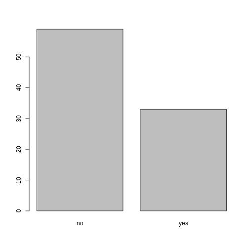
Looking at the plot compared to the output of the vector, we can see that in addition to “no”s and “yes”s, there are some respondents for whom the information about whether they were part of an irrigation association hasn’t been recorded, and encoded as missing data. These respondents do not appear on the plot. Let’s encode them differently so they can be counted and visualized in our plot.
R
## Let's recreate the vector from the data frame column "memb_assoc"
memb_assoc <- interviews$memb_assoc
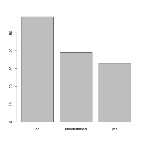
## replace the missing data with "undetermined"
memb_assoc[is.na(memb_assoc)] <- "undetermined"
## convert it into a factor
memb_assoc <- as.factor(memb_assoc)
## let's see what it looks like
memb_assoc
OUTPUT
  [1] undetermined yes          undetermined undetermined undetermined
  [6] undetermined no           yes          no           no
 [11] undetermined yes          no           undetermined yes
 [16] undetermined undetermined undetermined undetermined undetermined
 [21] no           undetermined undetermined no           no
 [26] no           undetermined no           yes          undetermined
 [31] undetermined yes          no           yes          yes
 [36] yes          undetermined yes          undetermined yes
 [41] undetermined no           no           undetermined no
 [46] no           yes          undetermined undetermined yes
 [51] undetermined no           yes          no           undetermined
 [56] yes          no           no           undetermined no
 [61] yes          undetermined undetermined undetermined no
 [66] yes          no           no           no           no
 [71] yes          undetermined no           yes          undetermined
 [76] undetermined yes          no           no           yes
 [81] no           no           yes          no           yes
 [86] no           no           undetermined yes          yes
 [91] yes          yes          yes          no           no
 [96] no           no           yes          no           no
[101] yes          yes          no           undetermined no
[106] no           undetermined no           no           undetermined
[111] no           undetermined undetermined no           no
[116] no           no           yes          no           no
[121] no           no           no           no           no
[126] no           no           no           no           yes
[131] undetermined
Levels: no undetermined yes
R
## bar plot of the number of interview respondents who were
## members of irrigation association:
plot(memb_assoc)
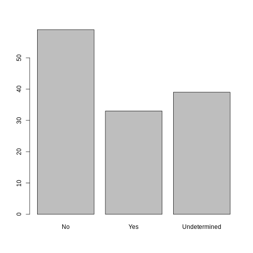
R
## Rename levels.
memb_assoc <- fct_recode(memb_assoc, No = "no",
                         Undetermined = "undetermined", Yes = "yes")
## Reorder levels. Note we need to use the new level names.
memb_assoc <- factor(memb_assoc, levels = c("No", "Yes", "Undetermined"))
plot(memb_assoc)
Formatting Dates
One of the most common issues that new (and experienced!) R users
have is converting date and time information into a variable that is
appropriate and usable during analyses. A best practice for dealing with
date data is to ensure that each component of your date is available as
a separate variable. In our dataset, we have a column
interview_date which contains information about the year,
month, and day that the interview was conducted. Let’s convert those
dates into three separate columns.
R
str(interviews)
We are going to use the package
lubridate, , which is included in the
tidyverse installation and should be
loaded by default. However, if we deal with older versions of tidyverse
(2022 and ealier), we can manually load it by typing
library(lubridate).
If necessary, start by loading the required package:
R
library(lubridate)
The lubridate function ymd() takes a vector representing
year, month, and day, and converts it to a Date vector.
Date is a class of data recognized by R as being a date and
can be manipulated as such. The argument that the function requires is
flexible, but, as a best practice, is a character vector formatted as
“YYYY-MM-DD”.
Let’s extract our interview_date column and inspect the
structure:
R
dates <- interviews$interview_date
str(dates)
OUTPUT
POSIXct[1:131], format: "2016-11-17" "2016-11-17" "2016-11-17" "2016-11-17" "2016-11-17" ...When we imported the data in R, read_csv() recognized
that this column contained date information. We can now use the
day(), month() and year()
functions to extract this information from the date, and create new
columns in our data frame to store it:
R
interviews$day <- day(dates)
interviews$month <- month(dates)
interviews$year <- year(dates)
interviews
OUTPUT
# A tibble: 131 × 17
   key_ID village  interview_date      no_membrs years_liv respondent_wall_type
    <dbl> <chr>    <dttm>                  <dbl>     <dbl> <chr>
 1      1 God      2016-11-17 00:00:00         3         4 muddaub
 2      2 God      2016-11-17 00:00:00         7         9 muddaub
 3      3 God      2016-11-17 00:00:00        10        15 burntbricks
 4      4 God      2016-11-17 00:00:00         7         6 burntbricks
 5      5 God      2016-11-17 00:00:00         7        40 burntbricks
 6      6 God      2016-11-17 00:00:00         3         3 muddaub
 7      7 God      2016-11-17 00:00:00         6        38 muddaub
 8      8 Chirodzo 2016-11-16 00:00:00        12        70 burntbricks
 9      9 Chirodzo 2016-11-16 00:00:00         8         6 burntbricks
10     10 Chirodzo 2016-12-16 00:00:00        12        23 burntbricks
# ℹ 121 more rows
# ℹ 11 more variables: rooms <dbl>, memb_assoc <chr>, affect_conflicts <chr>,
#   liv_count <dbl>, items_owned <chr>, no_meals <dbl>, months_lack_food <chr>,
#   instanceID <chr>, day <int>, month <dbl>, year <dbl>
Notice the three new columns at the end of our data frame.
In our example above, the interview_date column was read
in correctly as a Date variable but generally that is not
the case. Date columns are often read in as character
variables and one can use the as_date() function to convert
them to the appropriate Date/POSIXctformat.
Let’s say we have a vector of dates in character format:
R
char_dates <- c("7/31/2012", "8/9/2014", "4/30/2016")
str(char_dates)
OUTPUT
chr [1:3] "7/31/2012" "8/9/2014" "4/30/2016"We can convert this vector to dates as :
R
as_date(char_dates, format = "%m/%d/%Y")
OUTPUT
[1] "2012-07-31" "2014-08-09" "2016-04-30"Argument format tells the function the order to parse
the characters and identify the month, day and year. The format above is
the equivalent of mm/dd/yyyy. A wrong format can lead to parsing errors
or incorrect results.
For example, observe what happens when we use a lower case y instead of upper case Y for the year.
R
as_date(char_dates, format = "%m/%d/%y")
WARNING
Warning: 3 failed to parse.OUTPUT
[1] NA NA NAHere, the %y part of the format stands for a two-digit
year instead of a four-digit year, and this leads to parsing errors.
Or in the following example, observe what happens when the month and day elements of the format are switched.
R
as_date(char_dates, format = "%d/%m/%y")
WARNING
Warning: 3 failed to parse.OUTPUT
[1] NA NA NASince there is no month numbered 30 or 31, the first and third dates cannot be parsed.
We can also use functions ymd(), mdy() or
dmy() to convert character variables to date.
R
mdy(char_dates)
OUTPUT
[1] "2012-07-31" "2014-08-09" "2016-04-30"