Transform Data
Overview
Teaching: 40 min
Exercises: 25 minQuestions
What is tidy data?
How do I transfrom the data to the shape I need?
Objectives
Filter the rows and columns of your data using
dropandkeep.Calculate group statistics using
egen.Aggregate your data using
collapse.Change the way your data is organized using
reshape.
Filter data
There are many variables in our dataset loaded from data/raw/worldbank/WDICountry.csv.
. describe

Contains data
  obs:           263
 vars:            32
 size:       645,665
----------------------------------------------------------------------------------------------------------------------
              storage   display    value
variable name   type    format     label      variable label
----------------------------------------------------------------------------------------------------------------------
countrycode     str3    %9s                   Country Code
shortname       str50   %50s                  Short Name
tablename       str50   %50s                  Table Name
longname        str73   %73s                  Long Name
alphacode       str2    %9s                   2-alpha code
currencyunit    str42   %42s                  Currency Unit
specialnotes    str1294 %1294s                Special Notes
region          str26   %26s                  Region
incomegroup     str19   %19s                  Income Group
wb2code         str2    %9s                   WB-2 code
national~seyear str50   %50s                  National accounts base year
national~ceyear str9    %9s                   National accounts reference year
snapricevalua~n str36   %36s                  SNA price valuation
lendingcategory str9    %9s                   Lending category
othergroups     str9    %9s                   Other groups
systemofnatio~s str61   %61s                  System of National Accounts
alternativeco~r str22   %22s                  Alternative conversion factor
pppsurveyyear   str34   %34s                  PPP survey year
balanceofpaym~e str33   %33s                  Balance of Payments Manual in use
externaldebtr~s str11   %11s                  External debt Reporting status
systemoftrade   str20   %20s                  System of trade
governmentacc~t str31   %31s                  Government Accounting concept
imfdatadissem~d str51   %51s                  IMF data dissemination standard
latestpopulat~s str166  %166s                 Latest population census
latesthouseho~y str77   %77s                  Latest household survey
sourceofmostr~n str88   %88s                  Source of most recent Income and expenditure data
vitalregistra~e str48   %48s                  Vital registration complete
latestagricul~s str130  %130s                 Latest agricultural census
latestindustr~a int     %8.0g                 Latest industrial data
latesttradedata int     %8.0g                 Latest trade data
v31             byte    %8.0g
censusyear      float   %9.0g
----------------------------------------------------------------------------------------------------------------------
Sorted by:
     Note: Dataset has changed since last saved.
We will not use most of them, so let’s drop them.
drop specialnotes
drop alphacode currencyunit
In fact, we will keep fewer than we drop. There is a separate command for this complementary operation.
. keep countrycode shortname region incomegroup censusyear

. describe

Contains data
  obs:           263
 vars:             5
 size:        26,826
----------------------------------------------------------------------------------------------------------------------
              storage   display    value
variable name   type    format     label      variable label
----------------------------------------------------------------------------------------------------------------------
countrycode     str3    %9s                   Country Code
shortname       str50   %50s                  Short Name
region          str26   %26s                  Region
incomegroup     str19   %19s                  Income Group
censusyear      float   %9.0g
----------------------------------------------------------------------------------------------------------------------
Sorted by:
     Note: Dataset has changed since last saved.
Gotcha
The commands
keepanddropirreversibly change the data in your memory. Only use them if your work is easy to reproduce if you make an error, such as right after loading a dataset.
You can use variable name wildcards with both commands (drop latest*). Similarly, you can use the - character to keep or drop variables in the dataset. Stata will keep, or drop, all variables starting with the variable to the left of the - and ending with the variable to the right of the -.
To filter out observations, use drop if and keep if.
. count
  263

. drop if missing(incomegroup)
(46 observations deleted)

. count
  217
There are 46 fewer observations than before.
The command is the same as keep if !missing(incomegroup). The operator ! stands for negation, “not missing.”
Challenge
Keep countries with a population census more recent than 1999. How many countries have you dropped from the dataset?
Solution
Aggregate data
Calculate the number of countries in each income group and their average census year, using the egen command.
egen stands for “extended generate,” and it allows for creating statistics and other functions by groups.
. egen n_country = count(countrycode), by(incomegroup)
. egen average_census_year = mean(censusyear), by(incomegroup)
. describe

Contains data
  obs:           209
 vars:             7
 size:        22,990
----------------------------------------------------------------------------------------------------------------------
              storage   display    value
variable name   type    format     label      variable label
----------------------------------------------------------------------------------------------------------------------
countrycode     str3    %9s                   Country Code
shortname       str50   %50s                  Short Name
region          str26   %26s                  Region
incomegroup     str19   %19s                  Income Group
censusyear      float   %9.0g
n_country       float   %9.0g
average_censu~r float   %9.0g
----------------------------------------------------------------------------------------------------------------------
Sorted by:
     Note: Dataset has changed since last saved.
The command egen creates a new variable with the aggregated statistics.
There are many functions to be used in egen; count, min, max, sum and mean are the most commonly used.
You can group by multiple variables.
drop n_country
egen n_country = count(countrycode), by(incomegroup region)
Create a variable capturing the decade of the most recent population census and take its average by region.
generate census_decade = int(censusyear/10)*10
egen average_census_decade = mean(census_decade), by(region)
You can do this in one step, by nesting the function.
drop *census_decade
egen average_census_decade = mean(int(censusyear/10)*10), by(region)
Challenge
What does the following code do?
egen what_is_this_variable = sum(substr(incomegroup, 1, 4) == "High"), by(region)Solution
Challenge
Create a variable for the difference of
censusyearfrom the average of the region. Show that its mean is zero. Why?Solution
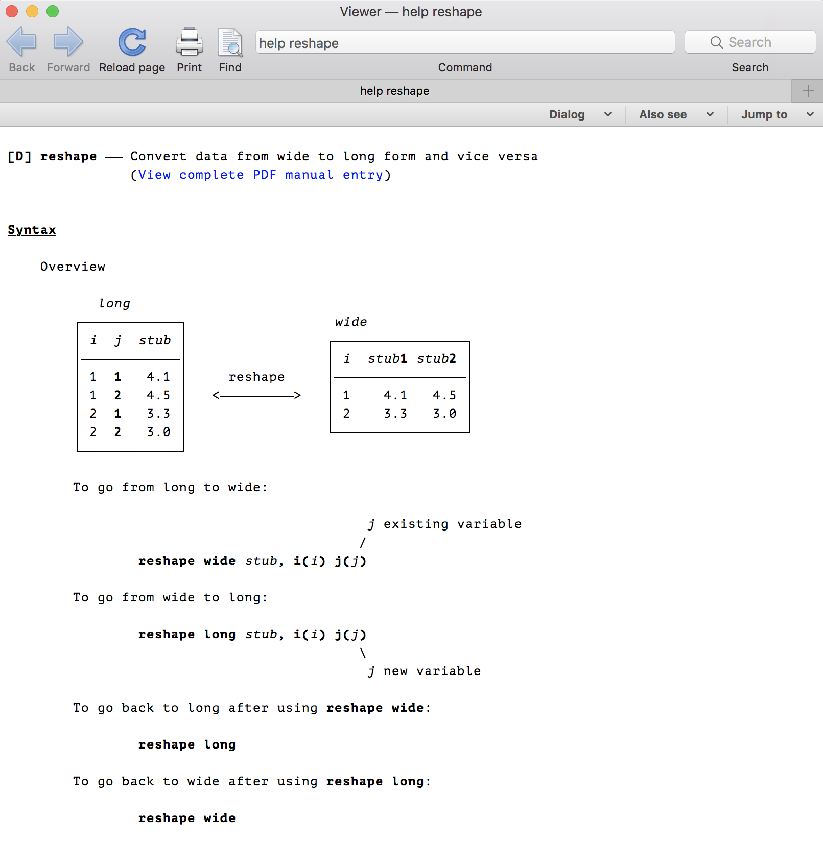
Reshape data
The WDI dataset has a strange shape. Variables are in separate rows, whereas years are in separate columns. This is the opposite of “tidy data,” where each variable has its own column, and different observations such as different years are in separate rows. We will reshape the data in the tidy format.
Different shapes of the data are useful for different tasks. For example, we may want to create a line graph from a variable. In Stata, this is only possible in years are in different observations (long form), not in different variables (wide form).
To practice reshaping, load a somewhat precleaned subset of the WDI dataset from the web. This will also show us how to work with data from the web. The data file we will be working with is located at https://raw.githubusercontent.com/korenmiklos/dc-economics-data/master/data/web/gdp.csv. Please go ahead and copy this URL from the shared notes so that you do not have to type it.
The command import delimited, but also use can load files directly from the web, if we pass them a URL. The URL has to be in quotes because it is full of strange characters.
import delimited "https://raw.githubusercontent.com/korenmiklos/dc-economics-data/master/data/web/gdp.csv", varnames(1) bindquotes(strict) encoding("utf-8") clear
browse
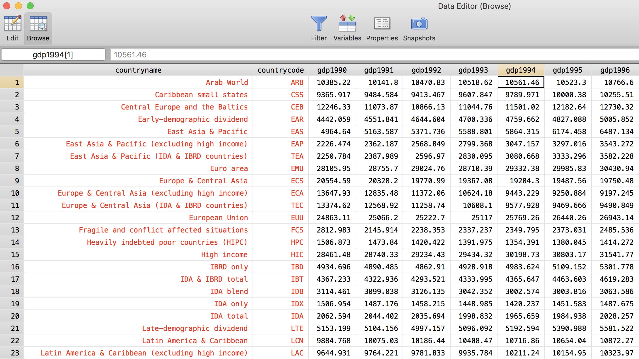
This data is too “wide”: column names contain information that we may want to work with. Let us reshape long.
. reshape long gdp, i(countrycode) j(year)
(note: j = 1990 1991 1992 1993 1994 1995 1996 1997 1998 1999 2000 2001 2002 2003 2004 2
> 005 2006 2007 2008 2009 2010 2011 2012 2013 2014 2015 2016 2017 2018)

Data                               wide   ->   long
-----------------------------------------------------------------------------
Number of obs.                      264   ->    7656
Number of variables                  31   ->       4
j variable (29 values)                    ->   year
xij variables:
            gdp1990 gdp1991 ... gdp2018   ->   gdp
-----------------------------------------------------------------------------
The option i() lists variables that index observations (rows) within the wide dataset. Each observation is a country in this wide format, so we use i(countrycode). We can have multiple variables inside i(), like i(countrycode countryname). The option j() gives one variable that indexes columns in the wide format. Because gdp1960, …, gdp2017 correspond to different years, we call this variable year.
The output of reshape is most helpful. After a reshape long, we have more observations and fewer variables. We see that we created a new variable called year (from the option j) and gdp1960, …, gdp2017 became a single variable, gdp.
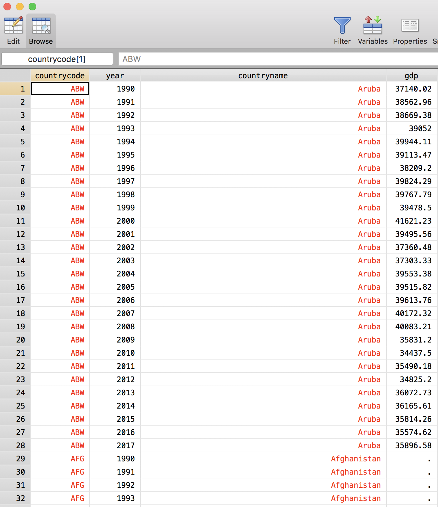
How does reshape know to look for gdp1960, …, gdp2017? Since we said reshape long gdp, ... it looks for variable names beginning with gdp and puts the remaining part of the variable name in the newly declared variable year. This is the most often used, default option, but we can also tell reshape what pattern to look for.
To undo this reshape,
. reshape wide gdp, i(countrycode) j(year)
(note: j = 1990 1991 1992 1993 1994 1995 1996 1997 1998 1999 2000 2001 2002 2003 2004 2
> 005 2006 2007 2008 2009 2010 2011 2012 2013 2014 2015 2016 2017 2018)

Data                               long   ->   wide
-----------------------------------------------------------------------------
Number of obs.                     7656   ->     264
Number of variables                   4   ->      31
j variable (29 values)             year   ->   (dropped)
xij variables:
                                    gdp   ->   gdp1990 gdp1991 ... gdp2018
-----------------------------------------------------------------------------
After a reshape, we can switch between the wide and long format more easily,
. reshape long
(note: j = 1990 1991 1992 1993 1994 1995 1996 1997 1998 1999 2000 2001 2002 2003 2004 2
> 005 2006 2007 2008 2009 2010 2011 2012 2013 2014 2015 2016 2017 2018)

Data                               wide   ->   long
-----------------------------------------------------------------------------
Number of obs.                      264   ->    7656
Number of variables                  31   ->       4
j variable (29 values)                    ->   year
xij variables:
            gdp1990 gdp1991 ... gdp2018   ->   gdp
-----------------------------------------------------------------------------
Optional
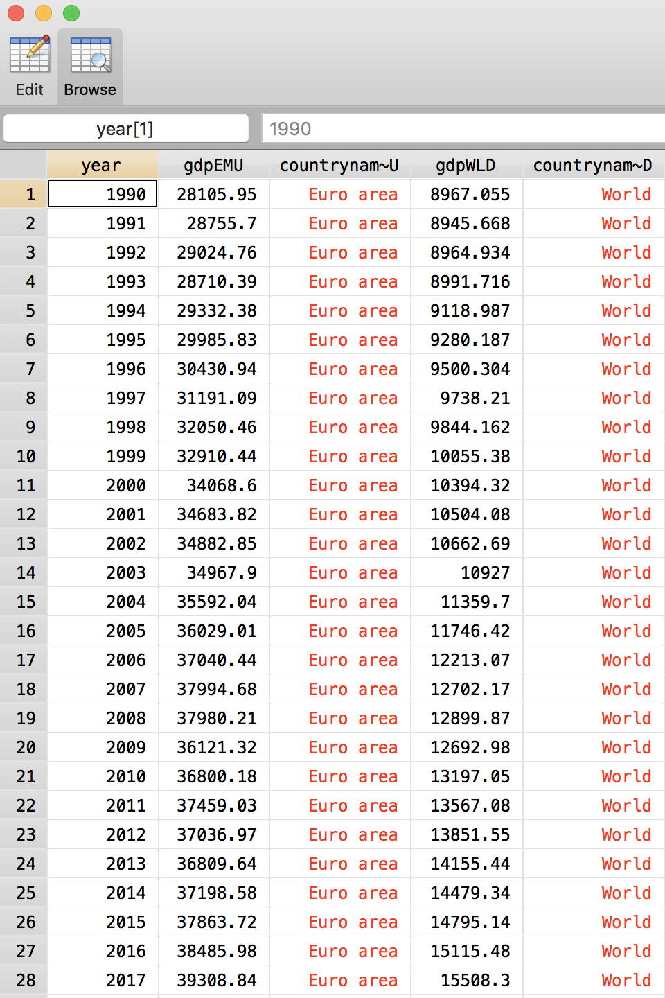
Suppose we want to compare Euro area GDP to World GDP for each year. For this, it would be great if these two series would be in different variables. We need a reshape wide.
. keep if inlist(countrycode, "EMU", "WLD")
(7,336 observations deleted)

. reshape wide gdp, i(year) j(countrycode)
variable countrycode is string; specify string option
r(109);
Ok, we can do that
. reshape wide gdp, i(year) j(countrycode) string
(note: j = EMU WLD)
variable countryname not constant within year
    Your data are currently long.  You are performing a reshape wide.  You typed something like

        . reshape wide a b, i(year) j(countrycode)

    There are variables other than a, b, year, countrycode in your data.  They must be constant within year because
    that is the only way they can fit into wide data without loss of information.

    The variable or variables listed above are not constant within year.  Perhaps the values are in error.  Type
    reshape error for a list of the problem observations.

    Either that, or the values vary because they should vary, in which case you must either add the variables to the
    list of xij variables to be reshaped, or drop them.
r(9);
The problem is that countryname also depends on countrycode and reshape does not know what to do with it. We can either reshape it, too, or drop it.
. reshape wide gdp countryname, i(year) j(countrycode) string
(note: j = EMU WLD)

Data                               long   ->   wide
-----------------------------------------------------------------------------
Number of obs.                       56   ->      28
Number of variables                   4   ->       5
j variable (2 values)       countrycode   ->   (dropped)
xij variables:
                                    gdp   ->   gdpEMU gdpWLD
                            countryname   ->   countrynameEMU countrynameWLD
-----------------------------------------------------------------------------
Challenge
Create a variable capturing the percentage deviation between Euro area GDP per capita and world GDP per capita.
Solution
Note that reshape changes the dataset in memory and you cannot undo it. Make sure you know what you are doing.
Save the steps
We will save this data in data/derived/gdp_per_capita.dta. It is good practice to keep data that we have derived from the original separate from the original, hence we need to create the folder derived inside data. We can use the shell command mkdir for this. After that, we can save the data, with a more informative name than gdp.
mkdir "data/derived"
save "data/derived/gdp_per_capita.dta"
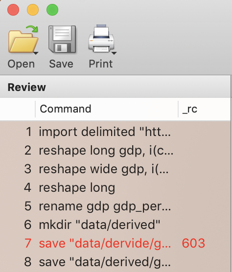
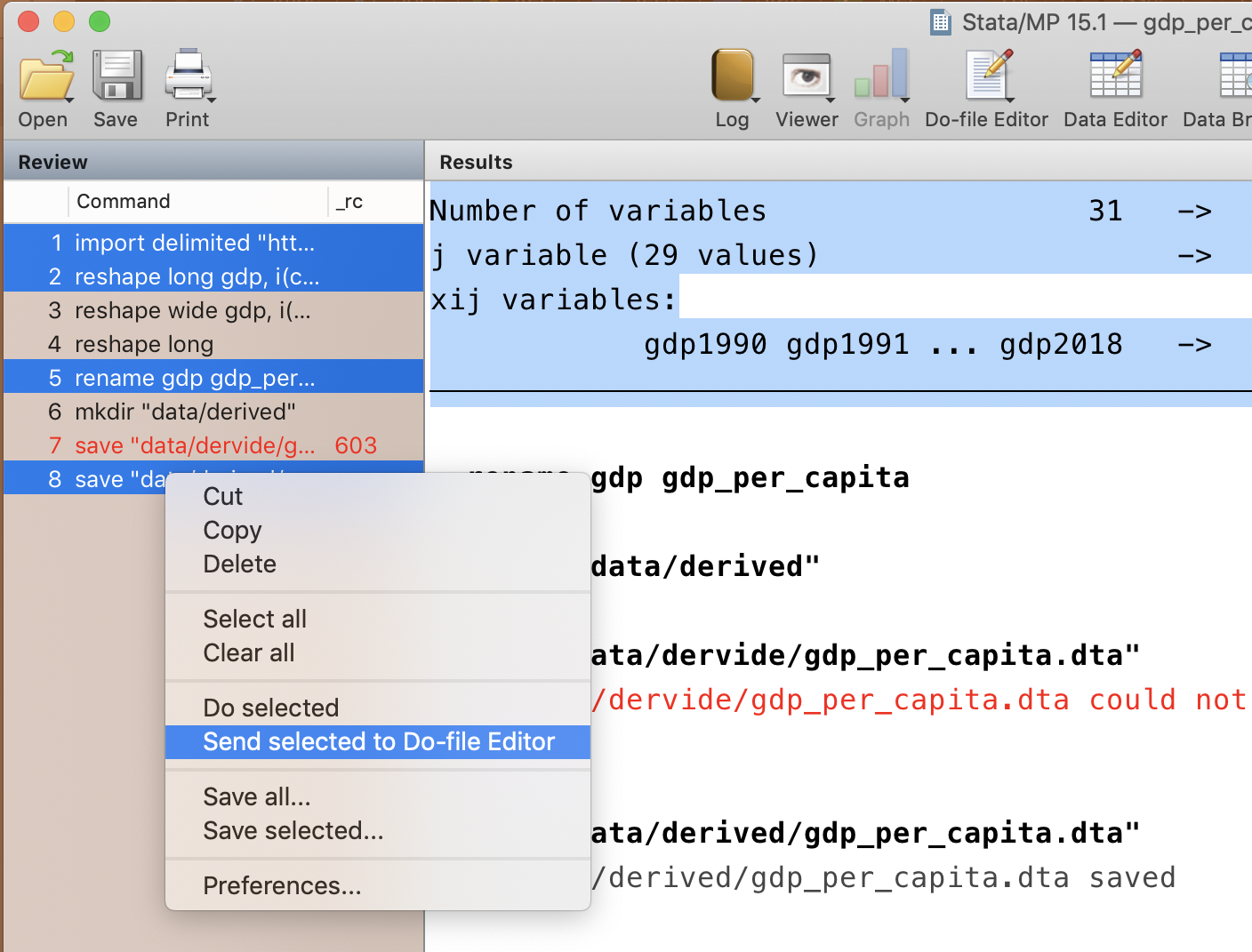
Commands that errored are red in the command history. Select the ones that we want to keep and send them to a .do file. We will not keep the mkdir command, because the folder has already been created and it would raise an error to try to create it again.
import delimited "https://raw.githubusercontent.com/korenmiklos/dc-economics-data/master/data/web/gdp.csv", varnames(1) bindquotes(strict) encoding("utf-8") clear
reshape long gdp, i(countrycode) j(year)
rename gdp gdp_per_capita
save "data/derived/gdp_per_capita.dta"
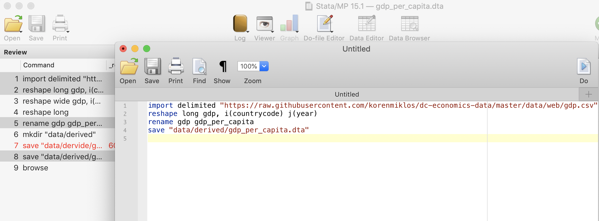
We save the file as code/read_reshape_gdp.do. Make sure you select the correct folder.
Challenge
Repeat the same loading, reshaping and saving steps with population data at
https://raw.githubusercontent.com/korenmiklos/dc-economics-data/master/data/web/pop.csv.Solution
Notice that there is a lot of repetition of code across the two files. You probably copied and pasted some code to solve the challenge. This poses a risk of errors if you forget to edit some copy-pasted code. In Episode 5, we will learn how to avoid repetition.
Key Points
Drop unnessecary variables freely.
Reshape your dataset to create tidy data.
Use
egento save statistics to new columns,collapseto aggregate the entire dataset.