Data Formats and Data Quality
Overview
Teaching: 40 min
Exercises: 25 minQuestions
How do I read tabular data?
How does Stata handle missing values?
Objectives
Import spreadsheet data.
Convert strings to numerical variables.
Deal with missing values.
Read a .csv file
Next we will read the World Development Indicators dataset. The data is in data/raw/worldbank/WDIData.csv.The other .csv files starting with WDI give some metadata. For example, data/raw/worldbank/WDISeries.csv describes the variables (“indicators” in World Bank speak), data/raw/worldbank/WDICountry.csv gives a codelist of countries, and data/raw/worldbank/WDIFootnote.csv includes footnotes.
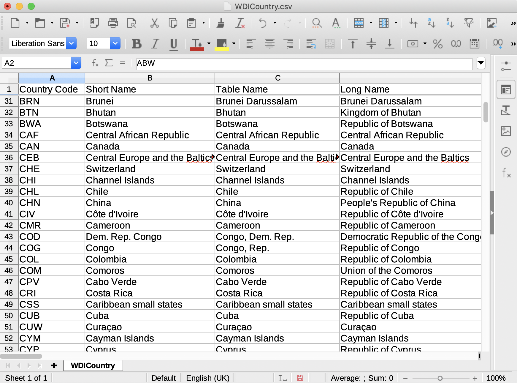
Reading text data from .csv files can be even more challenging. Let us read the country names and characteristics. This is what the file should look like.
import delimited "data/raw/worldbank/WDICountry.csv", varnames(1) clear
. import delimited "data/raw/worldbank/WDICountry.csv", varnames(1) clear
(31 vars, 268 obs)
As always, we look at the data first.
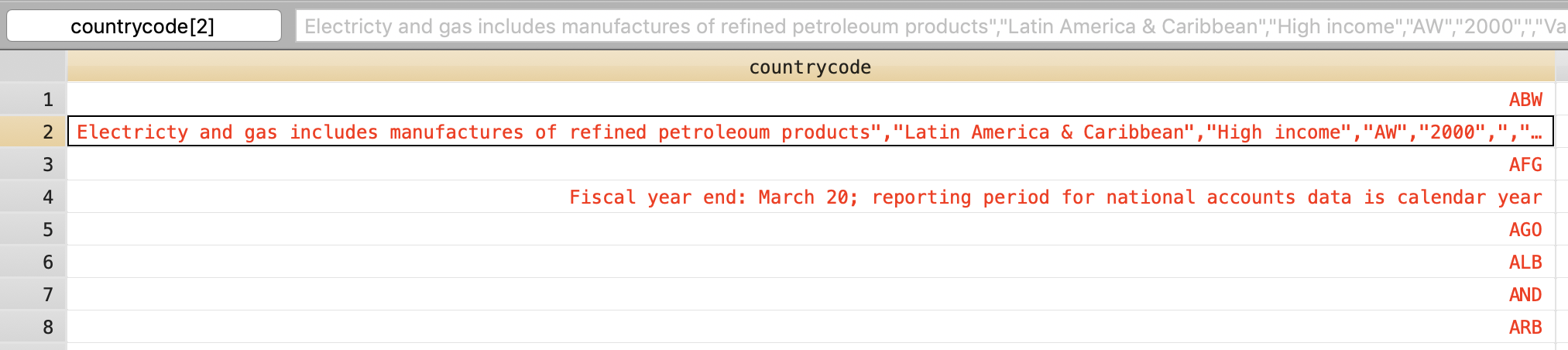
There are some things that do not belong to the countrycode variable. Indeed they look like entire parts of a .csv line.
After going out to the shell and exploring the file there (for example, head data/raw/worldbank/WDICountry.csv), we will find a text variable is split on multiple lines. This may trip up import delimited.
The following .csv cell, within double quotes, is spread across multiple lines.
"Central Bureau of Statistics and Central Bank of Aruba ; Source of population estimates: UN Population Division's World Population Prospects 2019 PROVISIONAL estimates. Not for circulation. Subject to change. Mining is included in agriculture\n
Electricty and gas includes manufactures of refined petroleum products"
We can tell import delimited to always looking for a closing quote before starting a new line with the bindquotes option.
. import delimited "data/raw/worldbank/WDICountry.csv", varnames(1) bindquotes(strict) clear
(31 vars, 263 obs)
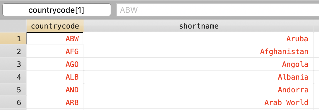
There are 5 fewer lines and the dataset looks fine.
But browsing further down, we find “Côte d’Ivoire” and “Curaçao” are misspelled.
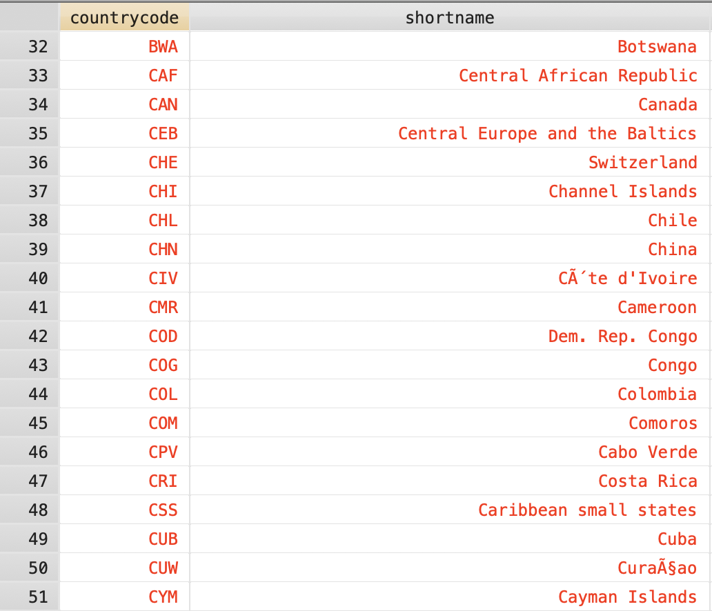
The characters à and Šare often indicative that the encoding of the text is UTF-8. We can set the encoding as an option to import delimited. The default encoding is latin1.
import delimited "data/raw/worldbank/WDICountry.csv", varnames(1) bindquotes(strict) encoding("utf-8") clear
Checking “Côte d’Ivoire” and “Curaçao,” we find the correct characters. The options varnames(1) bindquotes(strict) encoding("utf-8") are almost always necessary to properly read .csv files.
Variable types
Now all variables are read, but are variables of the proper type?
. codebook latestpopulationcensus

----------------------------------------------------------------------------------
latestpopulationcensus                                    Latest population census
----------------------------------------------------------------------------------

                  type:  string (str166)

         unique values:  34                       missing "":  46/263

              examples:  "1989"
                         "2010"
                         "2011"
                         "2014"

               warning:  variable has embedded blanks
From the examples, this looks like a numerical field, but is encoded as a 166-long string.
describe shows the type of each variable.
. describe

Contains data
  obs:           263
 vars:            31
 size:       644,613
----------------------------------------------------------------------------------------------------------------------
              storage   display    value
variable name   type    format     label      variable label
----------------------------------------------------------------------------------------------------------------------
countrycode     str3    %9s                   Country Code
shortname       str50   %50s                  Short Name
tablename       str50   %50s                  Table Name
longname        str73   %73s                  Long Name
alphacode       str2    %9s                   2-alpha code
currencyunit    str42   %42s                  Currency Unit
specialnotes    str1294 %1294s                Special Notes
region          str26   %26s                  Region
incomegroup     str19   %19s                  Income Group
wb2code         str2    %9s                   WB-2 code
national~seyear str50   %50s                  National accounts base year
national~ceyear str9    %9s                   National accounts reference year
snapricevalua~n str36   %36s                  SNA price valuation
lendingcategory str9    %9s                   Lending category
othergroups     str9    %9s                   Other groups
systemofnatio~s str61   %61s                  System of National Accounts
alternativeco~r str22   %22s                  Alternative conversion factor
pppsurveyyear   str34   %34s                  PPP survey year
balanceofpaym~e str33   %33s                  Balance of Payments Manual in use
externaldebtr~s str11   %11s                  External debt Reporting status
systemoftrade   str20   %20s                  System of trade
governmentacc~t str31   %31s                  Government Accounting concept
imfdatadissem~d str51   %51s                  IMF data dissemination standard
latestpopulat~s str166  %166s                 Latest population census
latesthouseho~y str77   %77s                  Latest household survey
sourceofmostr~n str88   %88s                  Source of most recent Income and expenditure data
vitalregistra~e str48   %48s                  Vital registration complete
latestagricul~s str130  %130s                 Latest agricultural census
latestindustr~a int     %8.0g                 Latest industrial data
latesttradedata int     %8.0g                 Latest trade data
v31             byte    %8.0g
----------------------------------------------------------------------------------------------------------------------
Sorted by:
     Note: Dataset has changed since last saved.
countrycode is str3, a 3-letter string. alphacode is str2, a 2-letter code. latesttradedata is int.
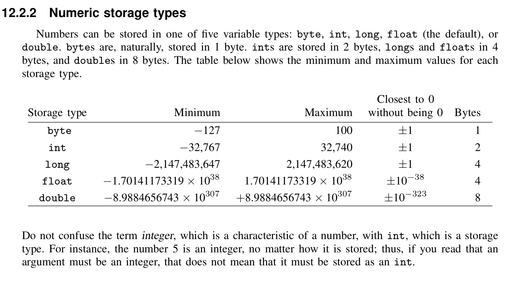
Year is an int, because it is less than 32,740 but greater than 100. When we create dummies (0/1 indicator variables), we can safely declare them as byte to save space.
generate byte low_income = (incomegroup == "Low income")
Beware of long integers, such as numerical identifiers. These may easily be greater than 32,740 and have to be declared as long.
generate long identifier = 12345678
Note that generate creates a new variable and we have filled it with a constant value, 12345678.
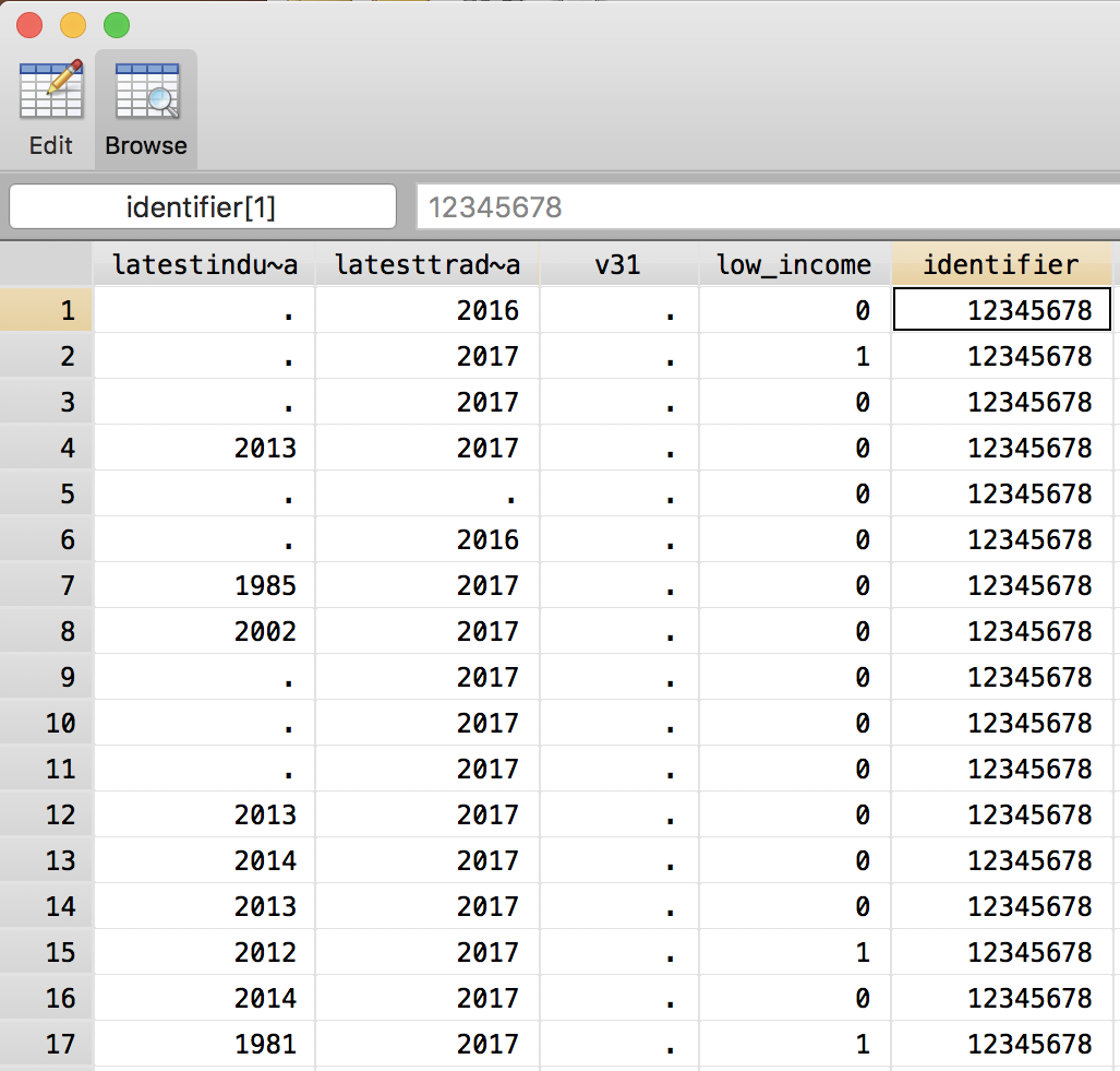
To give each observation its separate value, we need to use a function of other variables (like we defined low_income), read the data from a file, or merge a variable from another data file (see later). It is possible to change the value of a variable for a single observation, but why would you do that?
Identifiers sometimes have leading zeros, in which case it may be helpful to store them as string.
. generate str leading_zero_id = 01234567
type mismatch
r(109);
Strings always have to encapsulated in "".
. generate str leading_zero_id = "01234567"
Challenge
You have a fictive database named
balances.dtainUTF-8encoding. The database has a unique identifier variableceg_idin the third column. Ceg_id is the Company Registration Number which have possible zeros as a first character. You also have addresses variable which contains full firm adresses between double quotes, stored in a long string format. You have a dataset already loaded into your Stata.Please write an import delimited for this fictive balances.dta and read the ceg_id variable as a string variable. If you get stuck feel free to use the help of the
import delimitedcommand.Solution
import delimited balances.dta,varnames(1) stringcols(3) bindquotes(strict) encoding(“utf-8”) clear
Identifiers sometimes have leading zeros, in which case it may be helpful to read and store them as string and destring it later. The stringcols option only workes with the number of the column, you are not allowed to use the name of the variable inside the brackets.
Back to latestpopulationcensus. Because it looks like a numerical variable, we try to convert it from string.
. destring latestpopulationcensus, generate(censusyear)
latestpopulationcensus: contains nonnumeric characters; no generate
destring encountered an error (even if Stata does not display this as a red error message). What are the non-numeric values?
. tabulate latestpopulationcensus

               Latest population census |      Freq.     Percent        Cum.
----------------------------------------+-----------------------------------
                                   1943 |          1        0.46        0.46
                                   1979 |          1        0.46        0.92
                                   1984 |          2        0.92        1.84
                                   1987 |          1        0.46        2.30
                                   1989 |          1        0.46        2.76
                                   1997 |          1        0.46        3.23
                                   2001 |          1        0.46        3.69
                                   2002 |          2        0.92        4.61
                                   2003 |          2        0.92        5.53
                                   2004 |          2        0.92        6.45
                                   2005 |          2        0.92        7.37
                                   2006 |          3        1.38        8.76
                                   2007 |          3        1.38       10.14
                                   2008 |          7        3.23       13.36
                                   2009 |         11        5.07       18.43
2009. Population data compiled from a.. |          1        0.46       18.89
                                   2010 |         37       17.05       35.94
2010. Population data compiled from a.. |          1        0.46       36.41
2010. Population data compiled from a.. |          3        1.38       37.79
                                   2011 |         40       18.43       56.22
2011. Population data compiled from a.. |          9        4.15       60.37
2011. Population data compiled from a.. |          6        2.76       63.13
2011. Population figures compiled fro.. |          1        0.46       63.59
                                   2012 |         16        7.37       70.97
2012. Population data compiled from a.. |          2        0.92       71.89
                                   2013 |          7        3.23       75.12
                                   2014 |         11        5.07       80.18
                                   2015 |         12        5.53       85.71
2015. Population data compiled from a.. |          1        0.46       86.18
                                   2016 |         13        5.99       92.17
                                   2017 |         11        5.07       97.24
                                   2018 |          4        1.84       99.08
2018. Population data compiled from a.. |          1        0.46       99.54
          Guernsey: 2015; Jersey: 2011. |          1        0.46      100.00
----------------------------------------+-----------------------------------
                                  Total |        217      100.00
We can force destring to ignore these non-numeric entries (this may not be such a great idea).
. destring latestpopulationcensus, generate(censusyear) force
latestpopulationcensus: contains nonnumeric characters; censusyear generated as int
(72 missing values generated)

. tabulate censusyear, missing

     Latest |
 population |
     census |      Freq.     Percent        Cum.
------------+-----------------------------------
       1943 |          1        0.38        0.38
       1979 |          1        0.38        0.76
       1984 |          2        0.76        1.52
       1987 |          1        0.38        1.90
       1989 |          1        0.38        2.28
       1997 |          1        0.38        2.66
       2001 |          1        0.38        3.04
       2002 |          2        0.76        3.80
       2003 |          2        0.76        4.56
       2004 |          2        0.76        5.32
       2005 |          2        0.76        6.08
       2006 |          3        1.14        7.22
       2007 |          3        1.14        8.37
       2008 |          7        2.66       11.03
       2009 |         11        4.18       15.21
       2010 |         37       14.07       29.28
       2011 |         40       15.21       44.49
       2012 |         16        6.08       50.57
       2013 |          7        2.66       53.23
       2014 |         11        4.18       57.41
       2015 |         12        4.56       61.98
       2016 |         13        4.94       66.92
       2017 |         11        4.18       71.10
       2018 |          4        1.52       72.62
          . |         72       27.38      100.00
------------+-----------------------------------
      Total |        263      100.00
In general, we recommend against using force options with Stata commands as it might lead to errors.
The same non reversible process could happen if you use drop or keep commands. You might need to go back to the original dataset and read it in again. Drop eliminates variables or observations from the data in memory. Keep stores the variables that you specified in your varlist.
Instead of using force option we can write a function that extracts the year from the text. The function substr extracts a portion of a string variable. You must have to give three domains substr(s,n1,n2) to specify your command appropriately.
. display substr("apple", 1, 3)
app
You can see from this example that the first s domain was a string, the second n1 was a real number and the third n2 was an other real number. The n1 is the starting character, and n2 is the length of the string in characters.
Now we can generate a new year variable by the help of the substr function and the latestpopulationcensus string variable.
. drop censusyear

. generate censusyear_string = substr(latestpopulationcensus, 1, 4)
(46 missing values generated)

. generate censusyear = real(censusyear_string)
(47 missing values generated)

. tabulate censusyear, missing

 censusyear |      Freq.     Percent        Cum.
------------+-----------------------------------
       1943 |          1        0.38        0.38
       1979 |          1        0.38        0.76
       1984 |          2        0.76        1.52
       1987 |          1        0.38        1.90
       1989 |          1        0.38        2.28
       1997 |          1        0.38        2.66
       2001 |          1        0.38        3.04
       2002 |          2        0.76        3.80
       2003 |          2        0.76        4.56
       2004 |          2        0.76        5.32
       2005 |          2        0.76        6.08
       2006 |          3        1.14        7.22
       2007 |          3        1.14        8.37
       2008 |          7        2.66       11.03
       2009 |         12        4.56       15.59
       2010 |         41       15.59       31.18
       2011 |         56       21.29       52.47
       2012 |         18        6.84       59.32
       2013 |          7        2.66       61.98
       2014 |         11        4.18       66.16
       2015 |         13        4.94       71.10
       2016 |         13        4.94       76.05
       2017 |         11        4.18       80.23
       2018 |          5        1.90       82.13
          . |         47       17.87      100.00
------------+-----------------------------------
      Total |        263      100.00
We can nest functions and write the conversion in one step
generate censusyear = real(substr(latestpopulationcensus, 1, 4))
Challenge
Compare the number of missing values in the tables above. Why are they different?
Solution
With the first method,
destringand the option force we have forced all values with non-numerical entries to be missing. This includes entries like “2011. Population data compiled from administrative registers.” The second method, converting the first four characters of the string to a number, can parse this entry as 2011 and these entries will not be missing.
Challenge
Extract the national accounts base year as a number from the text variable
nationalaccountsbaseyear. Use the first two and the last two digits so that “2008/09” is read as 2009. The functionsubstr(x, -2, 2)selects the last two characters of a stringx.Solution
. tabulate nationalaccountsbaseyear

            National accounts base year |      Freq.     Percent        Cum.
----------------------------------------+-----------------------------------
                                   1954 |          1        0.49        0.49
                                   1974 |          1        0.49        0.97
                                   1984 |          1        0.49        1.46
                                   1985 |          1        0.49        1.94
                                1986/87 |          1        0.49        2.43
                                   1990 |          4        1.94        4.37
                                   1992 |          1        0.49        4.85
                                   1994 |          1        0.49        5.34
                                   1996 |          1        0.49        5.83
                                   1997 |          2        0.97        6.80
                                   1998 |          1        0.49        7.28
                                   1999 |          2        0.97        8.25
                                   2000 |          9        4.37       12.62
                                2000/01 |          1        0.49       13.11
                                   2001 |          1        0.49       13.59
                             20015/2016 |          1        0.49       14.08
                                   2002 |          2        0.97       15.05
                                2002/03 |          1        0.49       15.53
                                   2003 |          1        0.49       16.02
                                   2004 |          5        2.43       18.45
                                   2005 |          9        4.37       22.82
                                2005/06 |          2        0.97       23.79
                                   2006 |         16        7.77       31.55
                                   2007 |         15        7.28       38.83
                                   2008 |          2        0.97       39.81
                                2008/09 |          1        0.49       40.29
                                   2009 |          6        2.91       43.20
                                2009/10 |          1        0.49       43.69
                                   2010 |         25       12.14       55.83
                                   2011 |          5        2.43       58.25
                                2011/12 |          2        0.97       59.22
                                   2012 |          5        2.43       61.65
                                   2013 |          5        2.43       64.08
                                   2014 |          4        1.94       66.02
                                   2015 |          4        1.94       67.96
Original chained constant price data .. |         66       32.04      100.00
----------------------------------------+-----------------------------------
                                  Total |        206      100.00

. generate national_accounts_base_year = real(substr(nationalaccountsbaseyear, 1, 2) + substr(nationalaccountsbaseyear, -2, 2))
(123 missing values generated)

. tabulate national_accounts_base_year, missing

national_ac |
counts_base |
      _year |      Freq.     Percent        Cum.
------------+-----------------------------------
       1954 |          1        0.38        0.38
       1974 |          1        0.38        0.76
       1984 |          1        0.38        1.14
       1985 |          1        0.38        1.52
       1987 |          1        0.38        1.90
       1990 |          4        1.52        3.42
       1992 |          1        0.38        3.80
       1994 |          1        0.38        4.18
       1996 |          1        0.38        4.56
       1997 |          2        0.76        5.32
       1998 |          1        0.38        5.70
       1999 |          2        0.76        6.46
       2000 |          9        3.42        9.89
       2001 |          2        0.76       10.65
       2002 |          2        0.76       11.41
       2003 |          2        0.76       12.17
       2004 |          5        1.90       14.07
       2005 |          9        3.42       17.49
       2006 |         18        6.84       24.33
       2007 |         15        5.70       30.04
       2008 |          2        0.76       30.80
       2009 |          7        2.66       33.46
       2010 |         26        9.89       43.35
       2011 |          5        1.90       45.25
       2012 |          7        2.66       47.91
       2013 |          5        1.90       49.81
       2014 |          4        1.52       51.33
       2015 |          4        1.52       52.85
       2016 |          1        0.38       53.23
          . |        123       46.77      100.00
------------+-----------------------------------
      Total |        263      100.00
Missing values
Missing values
When a numerical variable contains no information for a particular observation, either because data was not recorded or because its calculation was erroneous, its value becomes missing. This is a special value, different from all actual numbers with its special rules of arithmetic. (Missing or null values or “not-a-numbers” are denoted NaN, NULL, or None in other programming languages.)
As seen from the table above, Stata denotes missing values with . We can use the missing function to test if a variable or an expression returns a missing value.
. display missing(2018)
0

. display missing(.)
1
Remember, 0 means false, 1 means true.
Operations on missing values return a missing value. So do inadmissible mathematical operations.
. display missing(1 + 2 + .)
1

. display missing(4 / 0)
1
For strings, the empty string is treated as missing value.
. display missing("")
1

. display missing(".")
0
Gotcha
Missing values are greater than any number.
. display 2018 < .
1

. display 2018 > .
0
Count counts the number of observations specified after a conditional statement. No varlists or string variables allowed. If nothing specified after count it displays the total number of observations in the dataset.
Challenge
Count how many countries have had their population census later than 2008.
Solution
count if censusyear > 2008 & !missing(censusyear)gives you an answer of 187. If you usecount if censusyear > 2008, you get 234. This is because Stata treats missing values as larger than any real number. It hence adds the 47 missing values.
Challenge
Which of the following tells you how many countries have more recent trade data than population census?
count if censusyear < latesttradedata
count if censusyear - latesttradedata < 0
count if latesttradedata - censusyear > 0
Solution
The second. When neither variable is missing, the three comparisons give the same answer. However, when
latesttradedatahas missing values, the first comparison evaluates to true, because missing values are greater than anything. The second comparison starts with a mathematical operation, which evaluates to missing and is hence not smaller than zero. As this property of missing values is a common gotcha, it is recommended to always explicitly test for missing values.count if censusyear < latesttradedata & !missing(censusyear, latesttradedata)
We are using the logical operators & (and), ! (not) and test for missing values in multiple variables. This latter returns 1 if any of the variables is missing.
Missing values are excluded from the statistical analyses by default; some commands will permit inclusion of missing values via options. Always be cautious when dealing with missing values and their replacement.
Challenge
Replace
national_accounts_base_yearwith the value extracted fromnationalaccountsreferenceyearif the former is missing but the latter is not.Solution
. replace national_accounts_base_year = real(substr(nationalaccountsreferenceyear, 1, 4)) if missing(national_accounts_base_year) & !missing(nationalaccountsreferenceyear)
(65 real changes made)
Key Points
Use the missing value feature of Stata, not a numerical code.
Test for missing values with the
missingfunction.In Stata expressions, missing values are greater than any number. Functions of missing values are missing value.
Check CSV files for separator, variable names, and character encoding.