- We’ve been working with the DTM data, which is the Digital Terrain Model, or the elevation of the ground
- LIDAR also collects data on the highest point in each location
- This is used to create a Digital Surface Model or DSM - the elevation of top physical point
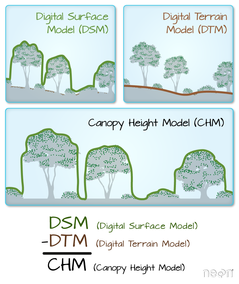
- In forested areas we can combine these to create a Canopy Height Model (CHM)
- Do this by subtracting the DTM from the DSM
library(stars)

dtm_harv <- read_stars("data/harv/harv_dtmcrop.tif")
dsm_harv <- read_stars("data/harv/harv_dsmcrop.tif")
chm_harv <- dsm_harv - dtm_harv
- Math happens on a cell by cell (elementwise) basis
- Can then graph this new raster
ggplot() +
  geom_stars(data = chm_harv)
- This lets us see where there are the tallest trees on the landscape and where there are none
Do Task 2 of Canopy Height from Space.