Spatial Data Vector

Remember to download and put into data subdirectory:

• LiDAR rasters and plot locations

Load the following into browser window:

• Projections picture

• So far we’ve worked with raster and vector data separately
• We’re using the stars package for raster data and the sf package for vector

library(ggplot2)
library(sf)
library(stars)

• We’ll also load ggplot2 again for plotting

• For raster data we’ve loaded it using read_stars and plotted it with geom_stars

dtm_harv <- read_stars("data/harv/harv_dtmCrop.tif")
ggplot() +
  geom_stars(data = dtm_harv)

• For vector data we’ve loaded it using read_sf and plotted it with geom_sf

plots_harv <- read_sf("data/harv/harv_plots.shp")
ggplot() +
  geom_sf(data = plots_harv)

• Now let’s plot them together

ggplot() +
  geom_stars(data = dtm_harv) +
  geom_sf(data = plots_harv)

• That wasn’t what we expected
• We don’t see the raster data and there appears to just be one point and an empty map
• Why?

Projections

• The reason this graph doesn’t work is that the two datasets have different projections
• We can see this by going back to the individual plots
• The axes on the vector plot latitude and longitude values in degrees, with numbers in the low 40s and low 70s
• The axes on the raster plot are much different, with values in the hundreds of thousands
• These differences are because the two sets of data have different “coordinate reference systems” or “projections”
• Since the earth is round we have to stretch geospatial data to present it on flat maps
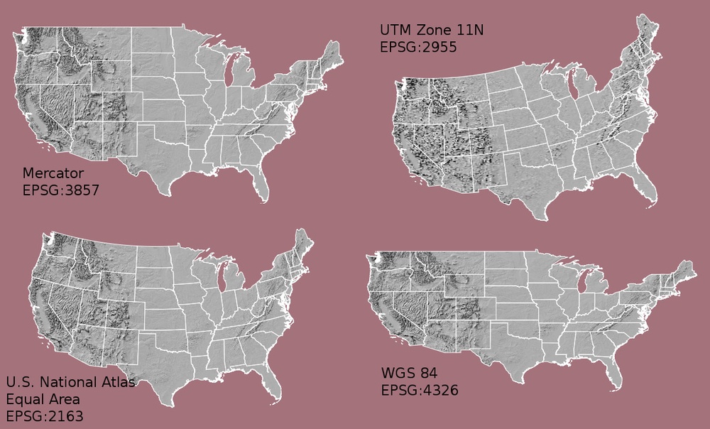
• There is no one best way to do this so there are different projects, which result in different representations of the world, and different units for locations
• Here are examples of a few common ones including two we’ll be working with WGS 84, which is latitude & longitude, and UTM

• The “coordinate reference system” or “CRS” indicates how this is done

• Coordinate Reference System (crs or projection) is different from raster.

• We can use st_crs to look up the CRS for this spatial data

st_crs(dtm_harv)

• The projection for the raster data is “UTM Zone 18N”

st_crs(plots_harv)

• The projection for the plots data is basically no projection, we’re using latitude and longitude

Transforming data into new projections

• To work with data having different projections together we can transform the projections to match each other
• Do this using the st_transform function
• Takes two arguments
• The geospatial object to be transformed
• The CRS to transform it to
• There are a variety of ways to indicate a CRS
• Including numeric codes and “well known text” of WKT representations for different coordinate reference systems
• Look at the CRS for dtm_harv
• See WKT
• Copy numeric EPSG code

plots_harv_utm <- st_transform(plots_harv, 32618)
st_crs(plots_harv_utm)

• Often the easiest thing to do when combining geospatial data is to match all objects to one of the existing CRS’s
• Do this by running st_crs on the object whose CRS you want to match
• So we’ll transform our plots data to have the same CRS as our vector data

plots_harv_utm <- st_transform(plots_harv, st_crs(dtm_harv))

• Because these two objects now have the same CRS the plot will look like we’d hoped it would

ggplot() +
  geom_stars(data = dtm_harv) +
  geom_sf(data = plots_harv_utm)

What Projections to Use

• We’ve seen two of the most common CRS’s
• Because we’re flattening a sphere no projection is perfect for all circumstances
• When choosing a CRS you want to think about what aspects of the world you want to preserve, like distance or area
• UTM, which stands for Universal Transverse Mercator, is one of the most commonly used projections in ecological research
• It accuractely represents local geospatial information and preserves distance
• It is primarily designed to work within different zones and so isn’t generally used at scales larger than a state
• Lat-longs are a common way of collecting data, but don’t preserve any key aspects of the data
• The Azimuthal Equal Area projection maintains area, so if the amount of area being worked with is important it’s a good projection
• So, for most of you UTM within your research zone will be the right way to go
• If you work at larger scales think about what it is most important to preserve and look for a transformation that does that

Summary

• To represent geospatial information from the surface of the sphere-like earth we have to stretch it to make it flat
• We do this using projections and that are represented as “coordinate reference systems” or “CRS”
• The st_transform function can transform data from one CRS to another
• This is often important for working with multiple geospatial objects
• Thought in some cases geospatial tools will quietly handle reprojection for us
• UTM with an appropriate local zone is the most common CRS used in ecological research

Do Task 4 of Canopy Height from Space.