Remember to download and put into data subdirectory:
Load the following into browser window:
Set-up R Console:
library(raster)
library(ggplot2)
raster import and structure
- Spatial data is often organized in a
raster.- gridded format (like coordinates)
- each pixel is a value
- most remote sensing and environmental data
-
raster()import - DSM is Digital Surface Model: elevation of top physical point
- See diagram
dsm_harv <- raster("data/neon-airborne/harv_dsmCrop.tif")
- Metadata is important to describe the context of spatial data.
bandsprojectionunitsmin,max,mean
Plotting spatial data with ggplot
- Continue using what we’ve been learning
- Useful for making nice maps combined with other figures
Three steps (write on board):
- Do Spatial Work (just importing so far)
- Convert to Data Frame (this is what ggplot works with)
- Make Plots
- Convert using
as.data.frame(overloaded byrasterto convert spatial data)
dsm_harv_df = as.data.frame(dsm_harv, xy = TRUE)
head(dsm_harv_df)
- Can then plot using
geom_raster
ggplot() +
  geom_raster(data = dsm_harv_df,
              aes(x = x, y = y, fill = HARV_dsmCrop))
- Because this is a data frame we can treat raster values like they are part of a normal table
ggplot() +
  geom_histogram(data = dsm_harv_df,
                 aes(x = HARV_dsmCrop))
Do Task 1 of Canopy Height from Space.
raster math
Show > * Canopy Height Model picture
- The DSM data is a Digital Surface Model: elevation of top physical point
- DTM is Digital Terrain Model: elevation of the ground
- We can create a Canopy Height Model (CHM) by taking the difference between them
dtm_harv <- raster("data/neon-airborne/harv_dtmcrop.tif")
chm_harv <- dsm_harv - dtm_harv
- Math happens on a cell by cell (elementwise) basis
- Can then graph this new raster by following the three rules
-
- Already did spatial work
-
- Convert to data frame
chm_harv_df = as.data.frame(chm_harv, xy = TRUE)
-
- Make plot
ggplot() +
  geom_raster(data = _harv_df,
              aes(x = x, y = y, fill = layer))
Do Task 2 of Canopy Height from Space.
Import and reproject shapefiles
vectordata includes points, lines, and polygonsshapefilesare one main format- set of multiple files
- same name, different extensions
readOGR("directory", "file_name_without_extensions")- stores data in a single
data.frame - access ‘attributes’ similar to GIS software using
$file_name$site_id
- stores data in a single
- set of multiple files
library(rgdal)

plots_harv <- readOGR("data/neon-airborne/plot_locations",
                      "harv_plots")
- Plot
vectoron top ofraster
chm_harv_df = as.data.frame(chm_harv, xy = TRUE)
plots_harv_df = as.data.frame(plots_harv)
ggplot() +
  geom_raster(data = chm_harv_df,
              aes(x = x, y = y, fill = layer)) +
  geom_point(data = plots_harv_df,
             aes(x = coords.x1, y = coords.x2), color = "yellow")
-
Uh oh, nothing happened.
-
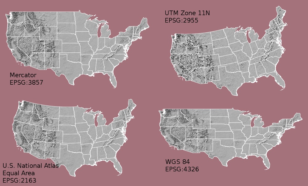
Coordinate Reference System (
crsorprojection) is different fromraster.
crs(chm_harv)
crs(plots_harv)
- Change projection:
- reproject
rasterwithprojectRaster() - reproject
vectorwithspTransform()
- reproject
plots_harv_utm <- spTransform(plots_harv, crs(chm_harv))
plots_harv_utm_df = as.data.frame(plots_harv_utm)
ggplot() +
  geom_raster(data = chm_harv_df,
              aes(x = x, y = y, fill = layer)) +
  geom_point(data = plots_harv_utm_df,
             aes(x = coords.x1, y = coords.x2), color = "yellow")
Do Task 3 of Canopy Height from Space.
Extract raster data
- Use
vectortoextract()values fromraster - These are canopy heights from
chm_harvat the coordinates fromplots_harv_utm.
plots_chm <- extract(chm_harv, plots_harv_utm)
- Order of values lines up with
plots_harv_utm$plot_id.
plots_harv_utm$plot_id
plots_chm <- data.frame(plot_num = plots_harv_utm$plot_id, plot_value = plots_chm)
- Often want values surrounding a point, not just the single pixel that the point lands in
- Do this using
bufferto get the values for all pixels within some buffer distance from the point
extract(chm_harv, plots_harv_utm, buffer = 10)
- This returns one value for each pixel within the buffer region
- Also what output is like for line and polygon data
-
One value for each cell intersected by a line or each cell inside a polygon
- Could keep all of this data, or calculate a value from it
- Often want an average
extract(chm_harv, plots_harv_utm, buffer = 10, fun = mean)
Do Tasks 4-5 of Canopy Height from Space.
Map of point data
- Maps are available in the
mapspackage - Maps are typically vector data
library(maps)
us_map = map_data("usa")
- Open
map - Polygons, but already stored as data frames (already done as.data.frame)
- Coordinates + Group + Order
- Group identifies unique polygons
- Order identifies how the points in each polygon are connected
- Draw a polygon illustrating points, edges, & order
ggplot() +
  geom_polygon(data = us_map,
               aes(x = long, y = lat, group = group),
               fill = "grey")
coord_quickmapgives us a reasonable projection
ggplot() +
  geom_polygon(data = us_map,
               aes(x = long, y = lat, group = group),
               fill = "grey") +
  coord_quickmap()
- Add other data on top
- Data on species occurances using the
spoccpackage - Gets data from multiple sources include GBIF
library(spocc)

do_gbif = occ(query = "Dipodomys ordii",
              from = "gbif",
              limit = 1000,
              has_coords = TRUE)
do_data = data.frame(dipo_df$gbif$data)
ggplot() +
  geom_polygon(data = us_map,
               aes(x = long, y = lat, group = group),
               fill = "grey") +
  geom_point(data = do_data,
             aes(x = Dipodomys_ordii.longitude,
                 y = Dipodomys_ordii.latitude)) +
  coord_quickmap()
Namespacing
library(dplyr)
library(raster)
raster’sselectfunction overwritesdplyr’sselectfunction- Demo error
select(do_data, Dipodomys_ordii.latitude)
- To use
dplyr’s function
dply::select(do_data, Dipodomys_ordii.latitude)
Making your own vector data
- Make spatial data from from non-spatial data with latitudes and longitudes
- Do to combine with other spatial data
- Need to know the
proj4stringfor standard latitude/longitude data "+proj=longlat +datum=WGS84 +ellps=WGS84 +towgs84=0,0,0"
points_crs <- crs("+proj=longlat +datum=WGS84 +ellps=WGS84 +towgs84=0,0,0")
do_data_spat <- SpatialPointsDataFrame(
	do_data[c('Dipodomys_ordii.longitude', 'Dipodomys_ordii.latitude')],
	do_data,
	proj4string = points_crs)
str(do_data_spat)
do_datawas a regular data frame, so do the same thing with your down data after loading it usingread_csv- Now you can do things like reproject and
extractvalues from rasters