Climate Space (Reproduction)
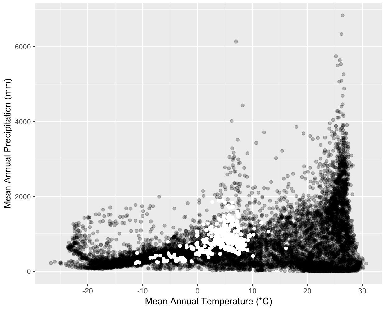
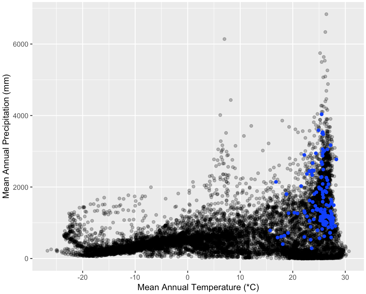
Understanding how environmental factors influence species distributions can be aided by determining which areas of the available climate space a species currently occupies. You are interested in showing how much and what part of the available global temperature and precipitation range is occupied by some common tree species. Create three graphs, one each for Quercus alba, Picea glauca, and Ceiba pentandra. Each graph should show a scatterplot of the mean annual temperature and mean annual precipitation for points around the globe and highlight the values for 1000 locations of the plant species. Start by decomposing this exercise into small manageable pieces.
Here are some tips that will be helpful along the way:
- Climate data data is available from the WorldClim
dataset. Using
climate <- getData('worldclim', var ='bio', res = 10)(from therasterpackage) will download all of the bioclim variables. The two variables you need arebio1(temperature) andbio12(precipitation). If the website is down you can download a copy from the course site by downloading http://www.datacarpentry.org/semester-biology/data/wc10.zip and unzipping it into your home directory (/home/usernameon Mac and Linux,C:\Users\username\Documentson Windows). - There are over 500,000 global data points which can make plotting slow. You
can choose to plot a random subset of 10,000 points (e.g., using
sample_nfrom thedplyrpackage) to limit the time it takes to generate. - Choose good labels and make the points transparent to see their density.
- You might notice that the temperature values seem large. Storing decimal values uses more space than integers, so the WorldClim creators provide temperature values multiplied by 10. For example, 19.5 is stored as 195. Make sure to display the actual temperatures, not the raw values provided.
- Species’ occurrence data is available from GBIF
using the
spoccpackage. An example of how to get the data you need is available in the Species Occurrences Map exercise. - To extract climate values for each occurrence from the climate data you will need a dataframe of occurrences that only only contains longitude and latitude columns.
- If the projections for WorldClim and the species occurrence data aren’t the same you will need a SpatialPointsDataframe.
- There are 19 bioclim variables that are stored together in a “raster stack”.
You can either: 1) run
extracton the full object returned bygetDataand then rundata.frameon the result. This will produce a table with one row for each species location and one column for each bioclim variable; or 2) Get the data for a single bioclim variable using the$, e.g.,climate$bio1, and run extract on this single raster.
Challenge (optional): If you want to challenge yourself trying making a single plot with all three species, either all on the same plot of split over three faceted subplots.
Expected outputs for Climate Space: 1 2 3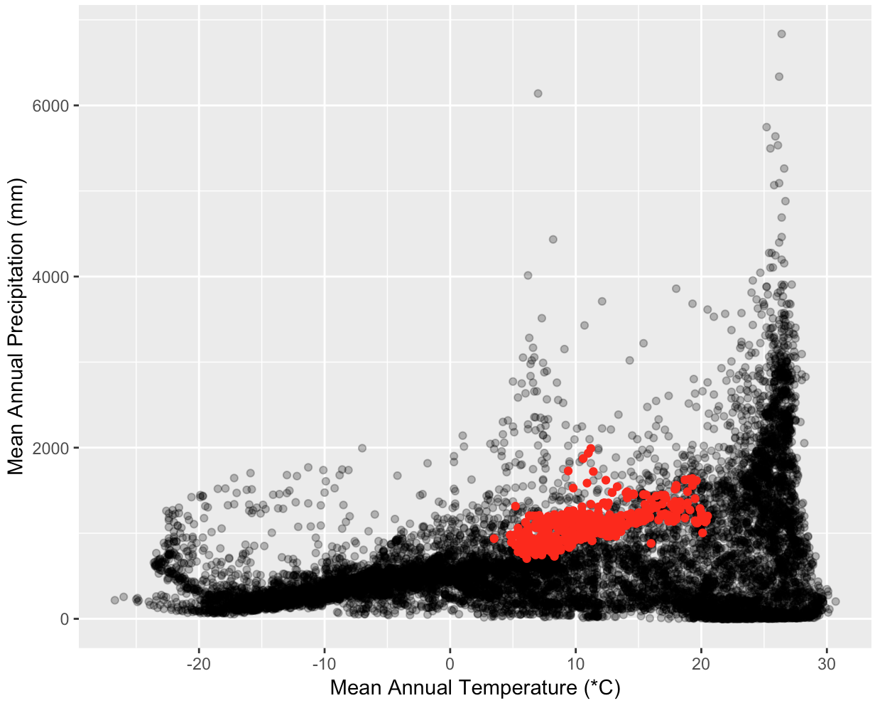