Tree Growth (Loops)
The UHURU experiment in Kenya has conducted a survey of Acacia and other tree species in ungulate exclosure treatments.
Each of the individuals surveyed were measured for tree height (HEIGHT), circumference (CIRC) and canopy size in two directions (AXIS_1 and AXIS_2).
If the file TREE_SURVEYS.txt isn’t already in your working directory,
download the data file here.
Read the data in using the following code:
tree_data <- read.csv("https://ndownloader.figshare.com/files/5629536",
                 sep = '\t',
                 na.strings = c("dead", "missing", "MISSING",
                                "NA", "?", "3.3."))
-
Write a function named
get_growth()that takes two inputs, a vector ofsizesand a vector ofyears, and calculates the average annual growth rate. Pseudo-code for calculating this rate is(size_in_last_year - size_in_first_year) / (last_year - first_year). Test this function by runningget_growth(c(40.2, 42.6, 46.0), c(2020, 2021, 2022)). -
Use dplyr and this function to get the growth for each individual tree along with information about the
TREATMENTthat tree occurs on. Trees are identified by a unique value in theORIGINAL_TAGcolumn. Don’t include information for cases where aTREATMENTis not known (e.g., where it isNA). -
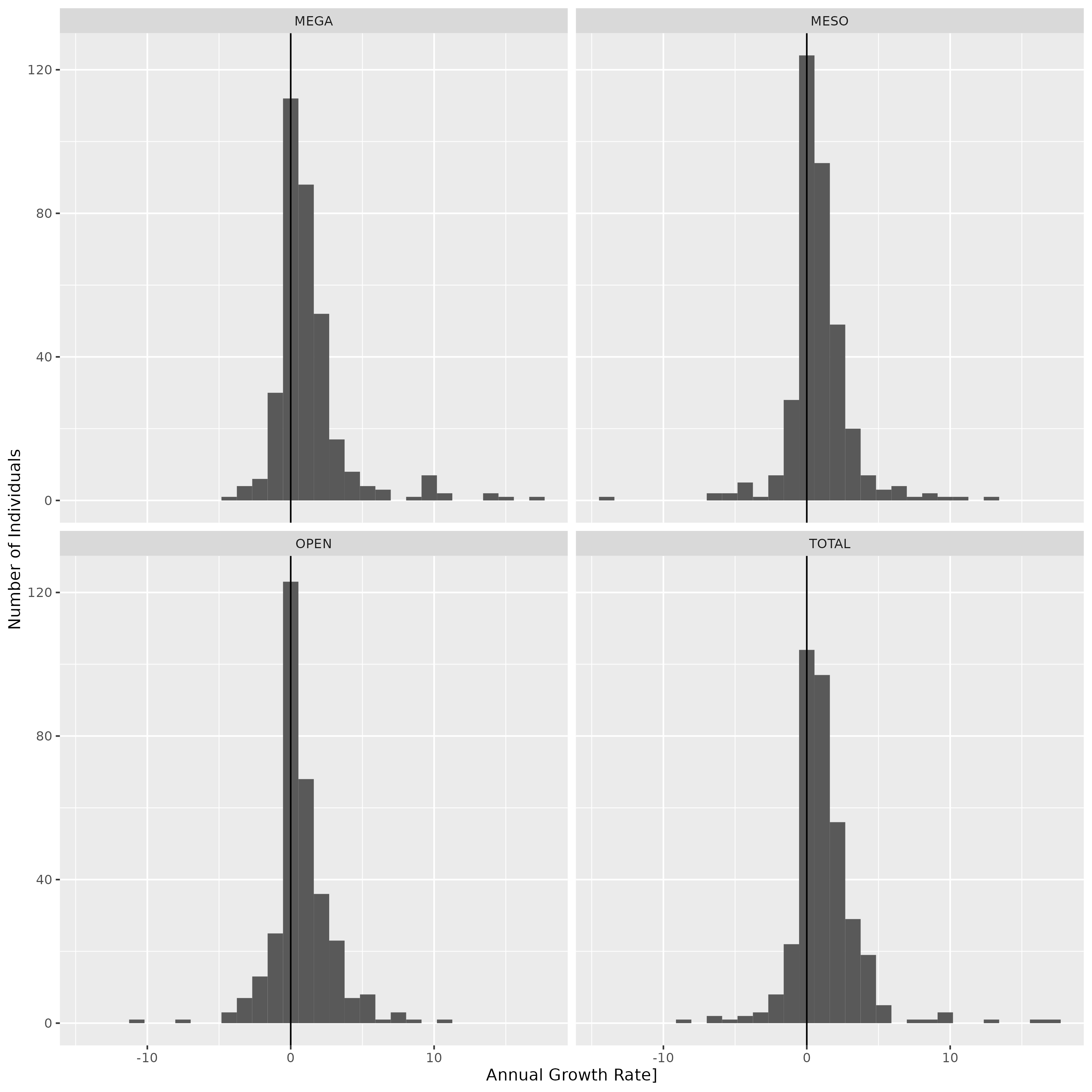
Using ggplot the output from (2) make a histogram of growth rates for each
TREATMENT, which eachTREATMENTin it’s own facet. Usegeom_vline()to add a vertical line at 0 to help indicate which trees are getting bigger vs. smaller. Include good axis labels. -
Create a single function called
compare_growth()that combines your work in (2) and (3). It should take the arguments:df(the data frame being used),measure(the column that contains the size measurement to measure growth on; we usedCIRC),tag_column(the name of the column with the unique tag; we usedORIGINAL_TAG),sample_column(the name of the column indicating different samples, we usedYEAR), andfacet_column(the name of the column to use to determine which groups to make histograms for, we usedTREATMENT). Use the function to recreate your original plot usingcompare_growth(tree_data, CIRC, ORIGINAL_TAG, YEAR, TREATMENT). Then use the function to create a similar plot showing growth facetedSPECIES, usingSURVEYas thesample_column, andAXIS_1as themeasureby runningcompare_growth(tree_data, AXIS_1, ORIGINAL_TAG, SURVEY, SPECIES).