Spatial Data 2

Learning Objectives

Following this assignment students should be able to:

• Map polygon data based on properties
• Aggregating raster data inside of polygons
• Crop and mask spatial data
• Save spatial data
• Create vector data based on locations data in csv files

Reading

Lecture Notes

Setup

install.packages(c("ggplot2", "stars", "sf"))
download.file("www.datacarpentry.org/semester-biology/data/neon-geospatial-data.zip", "neon-geospatial-data.zip", mode = "wb")
unzip("neon-geospatial-data.zip")
file.rename("neon-geospatial-data/", "data/")

Lectures

• Mapping polygon data based on properties
• Aggregating raster data inside polygons
• Why is ggplot plotting my UTM data as latitudes and longitudes and how do I make it stop
• Creating vector data from csv
• Cropping and Masking Spatial Data
• Saving Spatial Data From R

Place this code at the start of the assignment to load all the required packages.

library(stars)
library(sf)
library(ggplot2)
library(dplyr)

Exercises

1. Harvard Forest Soils Analysis (50 pts)

   The National Ecological Observatory Network has invested in high-resolution airborne imaging of their field sites. Elevation models generated from LiDAR can be used to map the topography and vegetation structure at the sites.

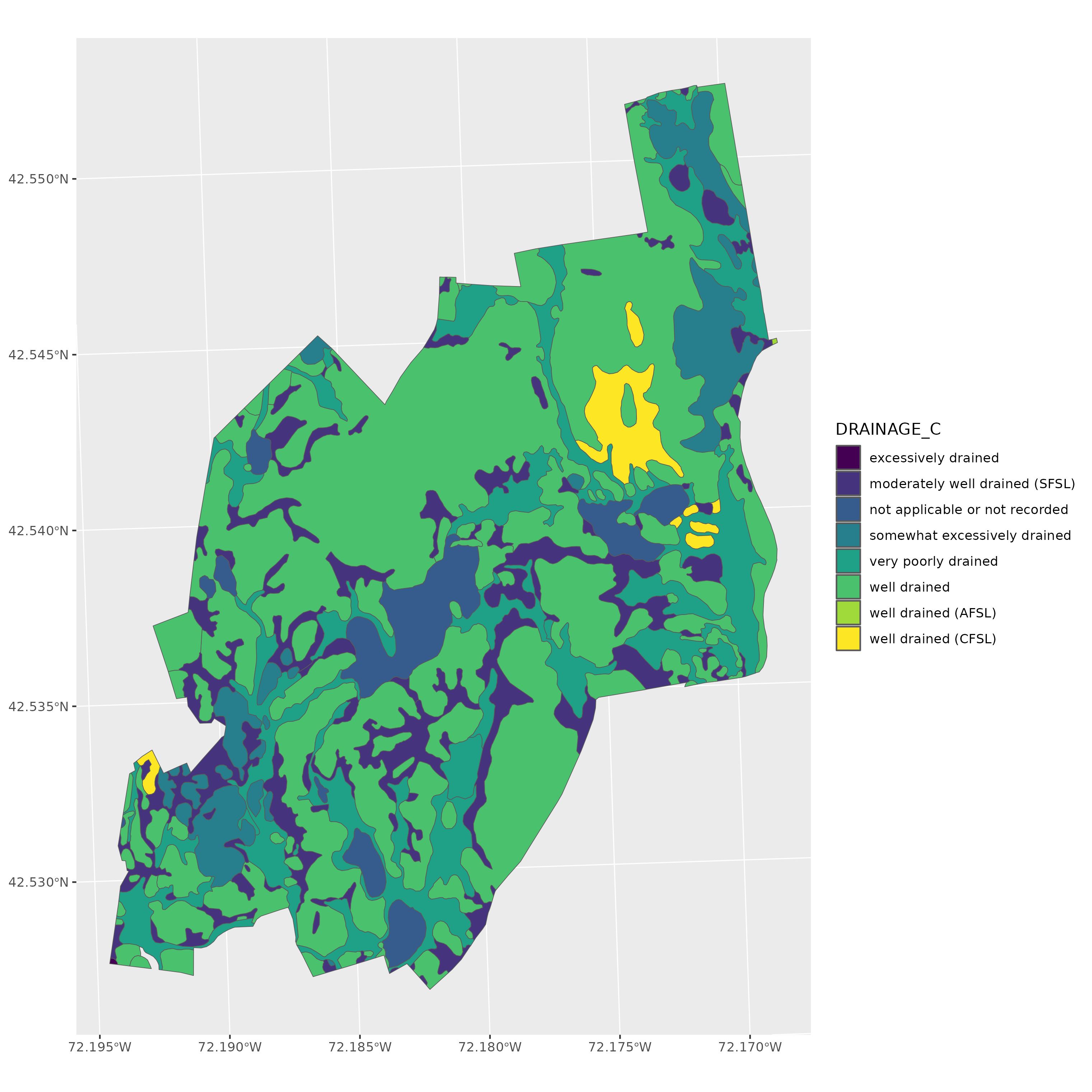
   Check to see if there is a data directory in your workspace with harv subdirectory in it. If not, Download the data and extract it into your working directory. The harv directory contains spatial data for Harvard Forest including raster data for a digital terrain model (harv_dtmfull.tif) and a digital surface model (harv_dsmfull.tif), and polygon data for the site boundary (harv_boundary.shp) and the soil types (harv_soils.shp).

   1. Make a map of the harv_soils data with the polygons colored based on DRAINAGE_C column. Use the viridis color ramp.
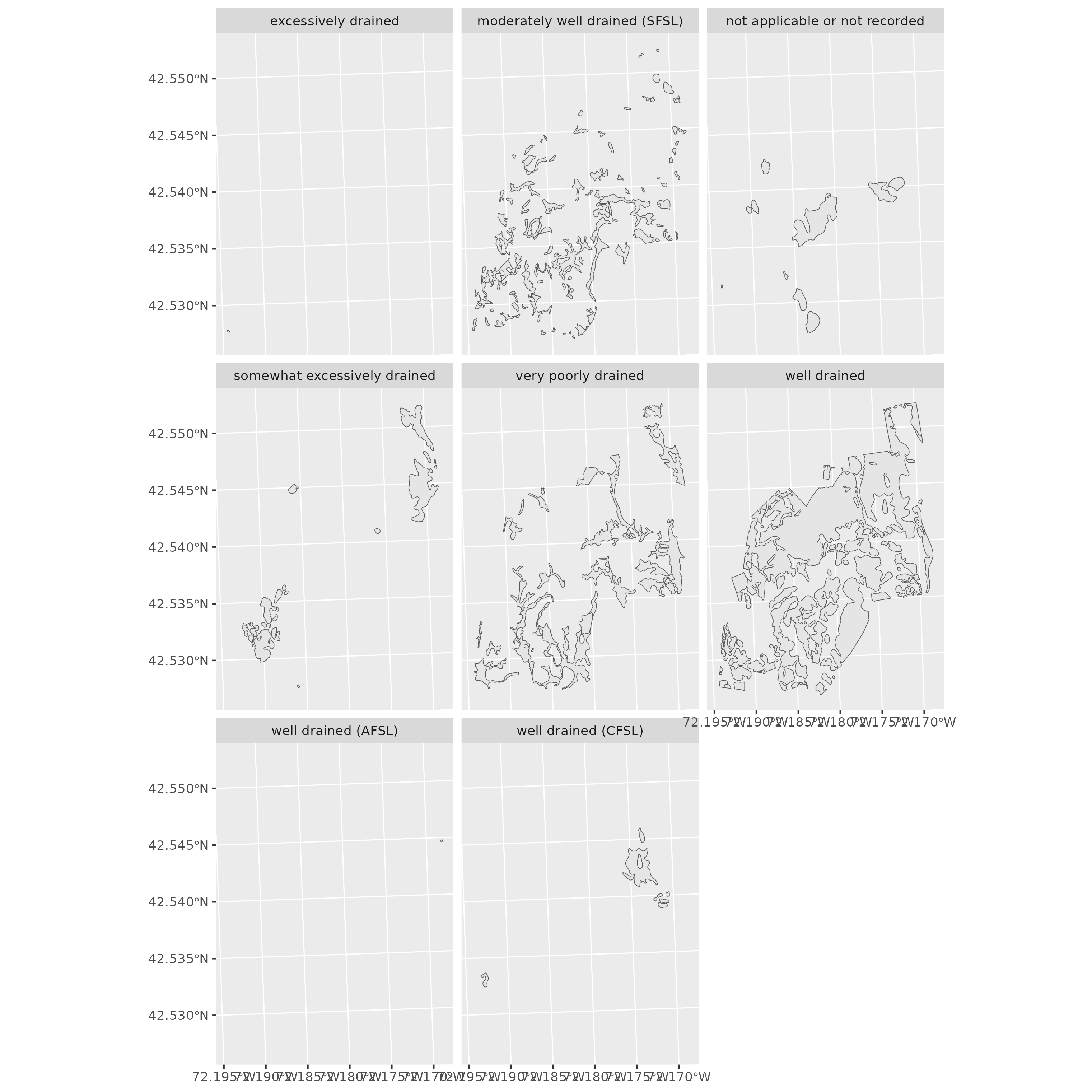
   2. Make a map of the harv_soils data with one facet (i.e., subplot) for each category in the DRAINAGE_C column.
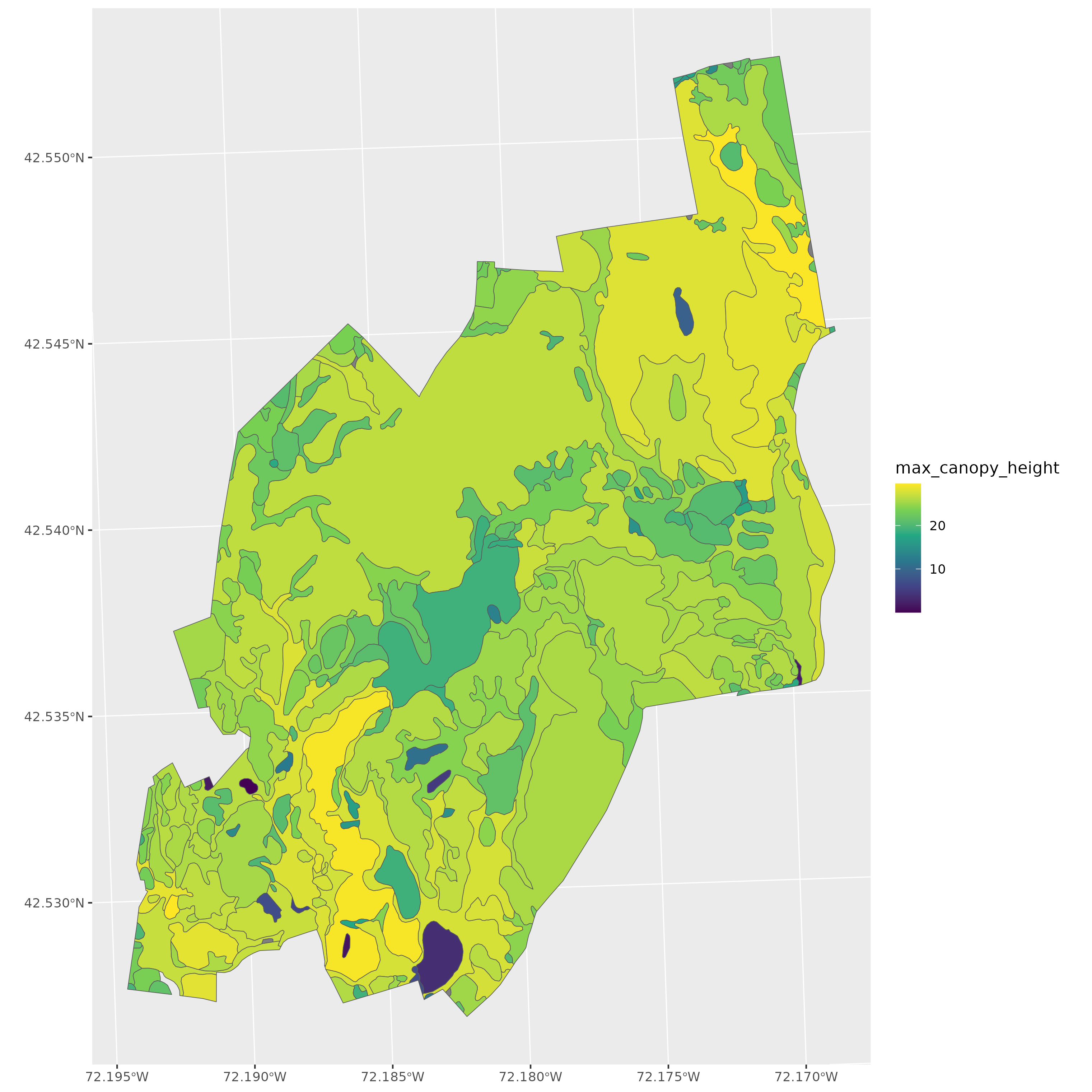
   3. Using the harv_dtmfull.tif and have_dsmfull.tif rasters create a canopy height model (DSM - DTM) and extract the maximum canopy height (i.e., the CHM value) within each soils polygon. To get the maximum canopy height instead of the mean value use the max function instead of mean. Display a vector of the resulting canopy height.
   4. Add the vector of canopy heights from (3) to the original sf object and display the resulting data frame.
   5. Make a map of the soil polygons colored based on their maximum canopy height. Use the viridis color ramp.
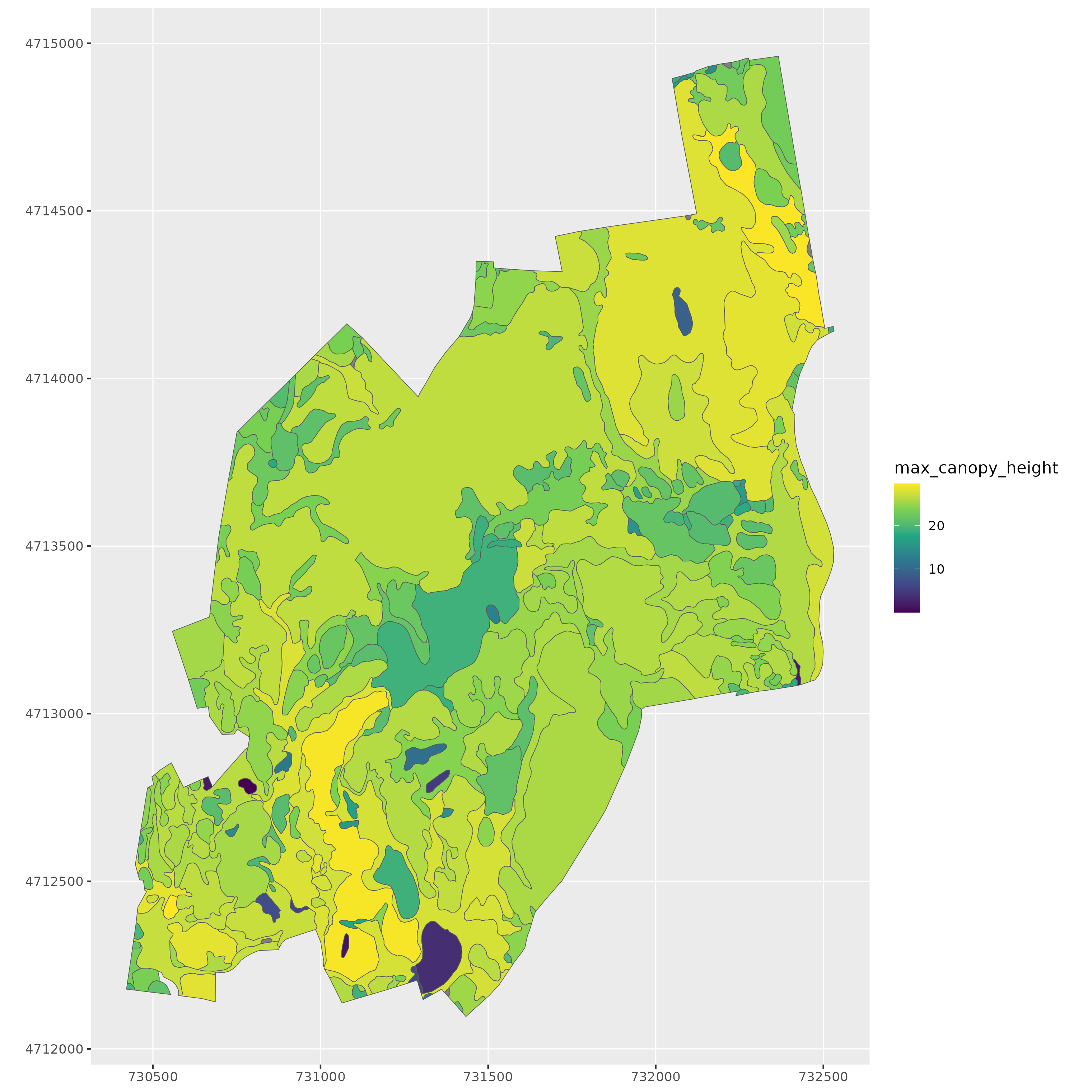
   6. Make a map that is the same as (5), but preserves the UTM coordinates on the axes.
   Expected outputs for Harvard Forest Soils Analysis: 1 2 3 4 5 6

2. Cropping NEON Data (50 pts)

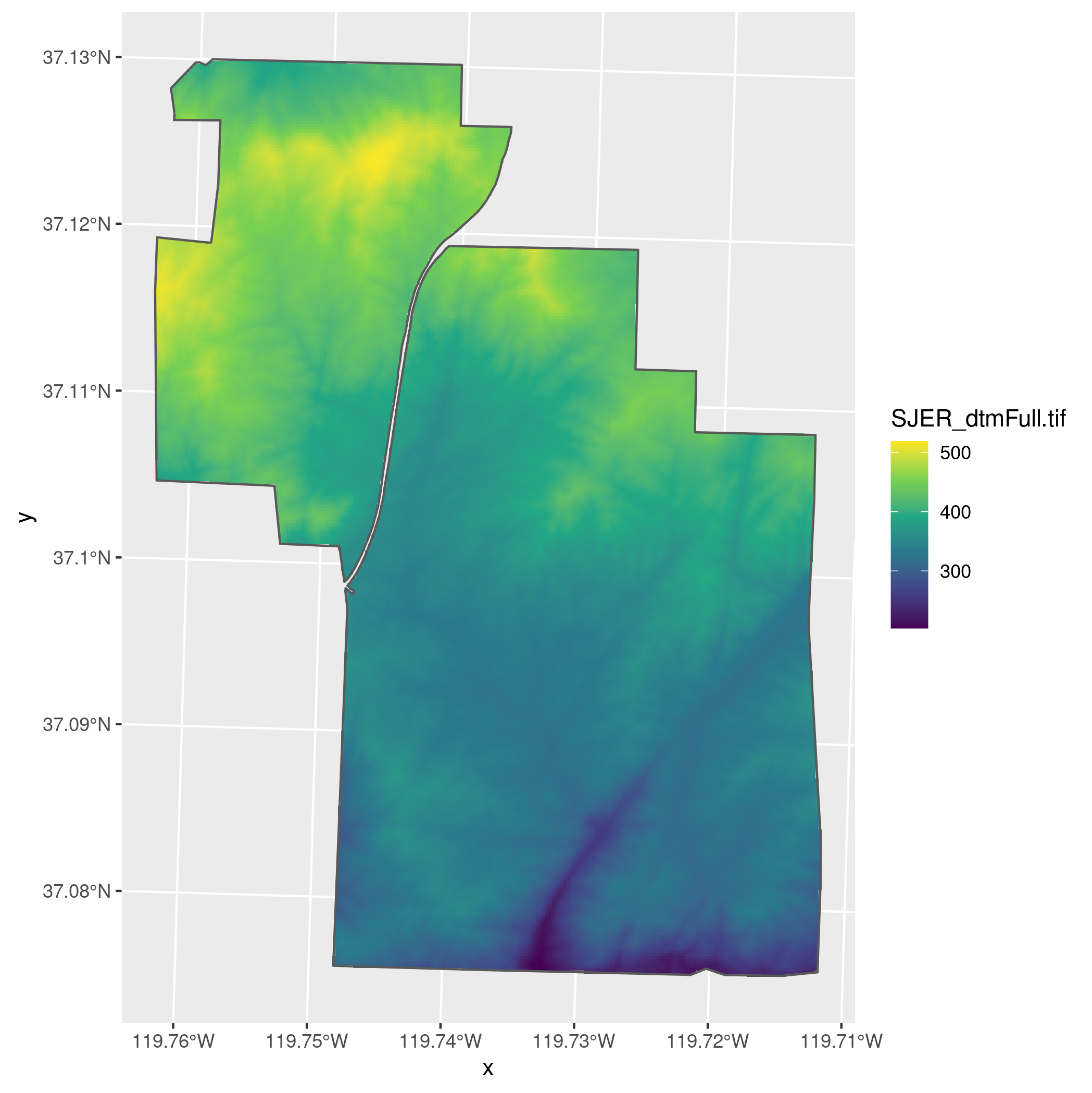
   The National Ecological Observatory Network has invested in high-resolution airborne imaging of their field sites. Elevation models generated from LiDAR can be used to map the topography and vegetation structure at the sites.

   Check to see if there is a data directory in your workspace with an SJER subdirectory in it. If not, Download the data and extract it into your working directory. The SJER directory contains csv data on plot locations (sjer_plots.csv), raster data for a digital terrain model (SJER_dtmFull.tif) and a digital surface model (SJER_dsmFull.tif), and vector data on the site boundary (sjer_boundary.shp) for the San Joaquin Experimental Range.

   1. Load the csv plots data (sjer_plots.csv) as an sf object and display that object (don’t load the shape files, use the csv file). The data is in latitudes and longitudes, so the CRS code is 4326.
   2. Reproject the plots data to the UTM coordinates of the DTM data (SJER_dtmFull.tif) and display the resulting object.
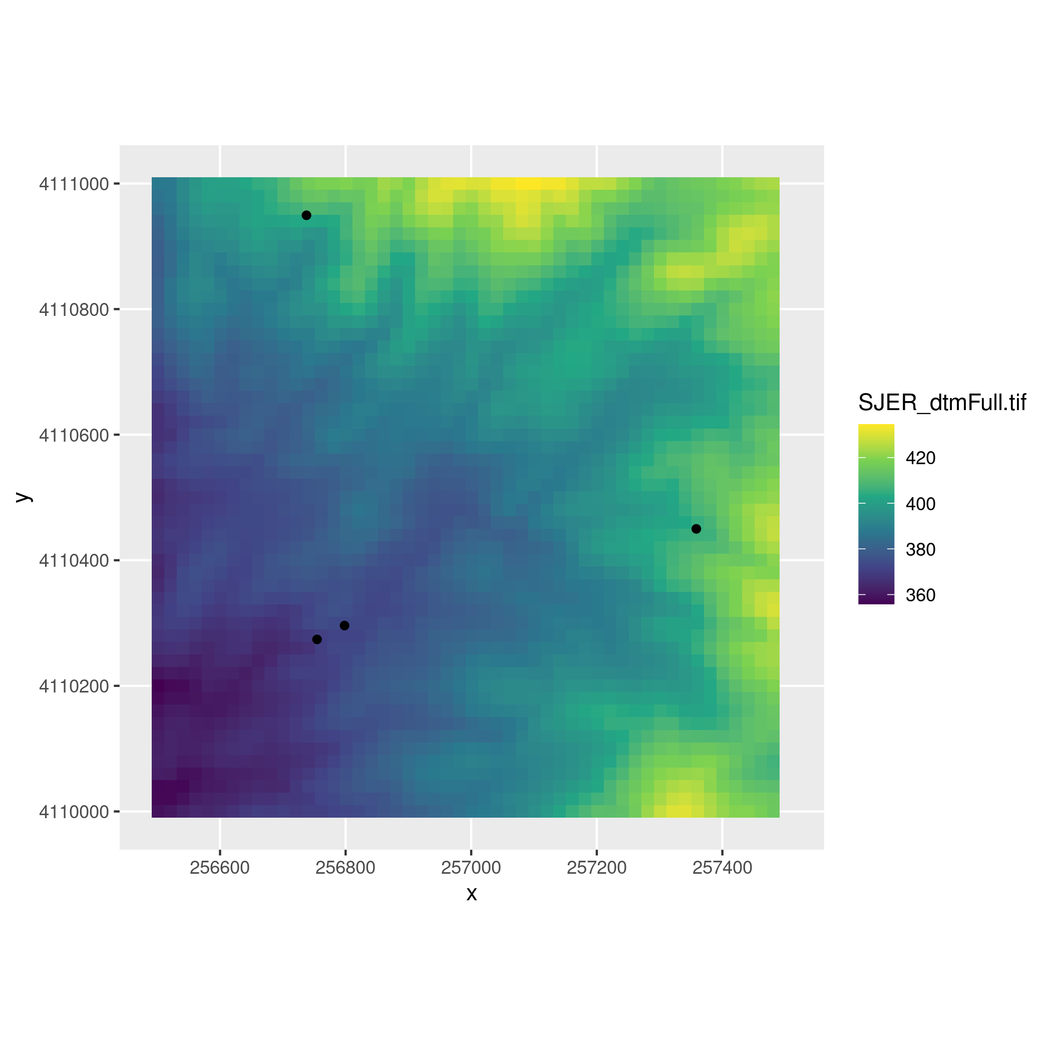
   3. Crop the DTM data to the site boundary (sjer_boundary.shp). To do this, first reproject the site boundary to have the same CRS as the DTM. Make a map showing the site boundary and the cropped DTM data without null values. Use the viridis color ramp.
   4. Use a bounding box to crop both the DTM data and the plots data. The bounding box should have xmin = 256500, xmax = 257500, ymin = 4110000, and ymax = 4111000. Make a map showing the cropped DTM (with no null values and the viridis color ramp) and the cropped points. Display the plot in the UTM coordinates.
   5. Save the map from (4) as an image named sjer_cropped_figure.png.
   6. Write the cropped DTM from (4) to a geotiff file. Name it sjer_dtm_cropped.tif. Write the cropped plots data from (4) to a shape file. Name it sjer_plots_cropped.shp.
   Expected outputs for Cropping NEON Data: 1 2 3

Assignment submission & checklist