Data Wrangling with tidyr
Last updated on 2025-04-01 | Edit this page
Overview
Questions
- How can I reformat a data frame to meet my needs?
Objectives
- Describe the concept of a wide and a long table format and for which purpose those formats are useful.
- Describe the roles of variable names and their associated values when a table is reshaped.
- Reshape a dataframe from long to wide format and back with the
pivot_widerandpivot_longercommands from thetidyrpackage. - Export a dataframe to a csv file.
dplyr pairs nicely with
tidyr which enables you to swiftly convert
between different data formats (long vs. wide) for plotting and
analysis. To learn more about tidyr after
the workshop, you may want to check out this handy
data tidying with tidyr
cheatsheet.
To make sure everyone will use the same dataset for this lesson, we’ll read again the SAFI dataset that we downloaded earlier.
R
## load the tidyverse
library(tidyverse)
library(here)

interviews <- read_csv(here("data", "SAFI_clean.csv"), na = "NULL")

## inspect the data
interviews

## preview the data
# view(interviews)
Reshaping with pivot_wider() and pivot_longer()
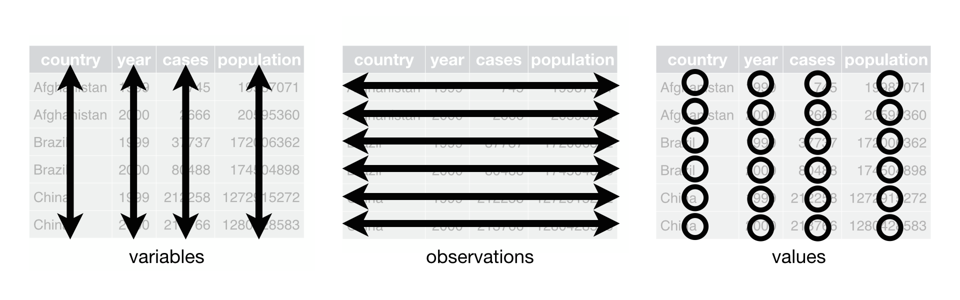
There are essentially three rules that define a “tidy” dataset:
- Each variable has its own column
- Each observation has its own row
- Each value must have its own cell
This graphic visually represents the three rules that define a “tidy” dataset:
 R for Data Science,
Wickham H and Grolemund G (https://r4ds.had.co.nz/index.html)
© Wickham, Grolemund 2017 This image is licenced under
Attribution-NonCommercial-NoDerivs 3.0 United States (CC-BY-NC-ND 3.0
US)
R for Data Science,
Wickham H and Grolemund G (https://r4ds.had.co.nz/index.html)
© Wickham, Grolemund 2017 This image is licenced under
Attribution-NonCommercial-NoDerivs 3.0 United States (CC-BY-NC-ND 3.0
US)
In this section we will explore how these rules are linked to the
different data formats researchers are often interested in: “wide” and
“long”. This tutorial will help you efficiently transform your data
shape regardless of original format. First we will explore qualities of
the interviews data and how they relate to these different
types of data formats.
Long and wide data formats
In the interviews data, each row contains the values of
variables associated with each record collected (each interview in the
villages). It is stated that the key_ID was “added to
provide a unique Id for each observation” and the
instanceID “does this as well but it is not as convenient
to use.”
Once we have established that key_ID and
instanceID are both unique we can use either variable as an
identifier corresponding to the 131 interview records.
R
interviews %>%
  select(key_ID) %>%
  distinct() %>%
  nrow()
OUTPUT
[1] 131As seen in the code below, for each interview date in each village no
instanceIDs are the same. Thus, this format is what is
called a “long” data format, where each observation occupies only one
row in the dataframe.
R
interviews %>%
  filter(village == "Chirodzo") %>%
  select(key_ID, village, interview_date, instanceID) %>%
  sample_n(size = 10)
OUTPUT
# A tibble: 10 × 4
   key_ID village  interview_date      instanceID
    <dbl> <chr>    <dttm>              <chr>
 1    192 Chirodzo 2017-06-03 00:00:00 uuid:f94409a6-e461-4e4c-a6fb-0072d3d58b00
 2     56 Chirodzo 2016-11-16 00:00:00 uuid:973c4ac6-f887-48e7-aeaf-4476f2cfab76
 3     37 Chirodzo 2016-11-17 00:00:00 uuid:408c6c93-d723-45ef-8dee-1b1bd3fe20cd
 4     49 Chirodzo 2016-11-16 00:00:00 uuid:2303ebc1-2b3c-475a-8916-b322ebf18440
 5     65 Chirodzo 2016-11-16 00:00:00 uuid:143f7478-0126-4fbc-86e0-5d324339206b
 6     35 Chirodzo 2016-11-17 00:00:00 uuid:ff7496e7-984a-47d3-a8a1-13618b5683ce
 7     47 Chirodzo 2016-11-17 00:00:00 uuid:2d0b1936-4f82-4ec3-a3b5-7c3c8cd6cc2b
 8     63 Chirodzo 2016-11-16 00:00:00 uuid:86ed4328-7688-462f-aac7-d6518414526a
 9      8 Chirodzo 2016-11-16 00:00:00 uuid:d6cee930-7be1-4fd9-88c0-82a08f90fb5a
10     53 Chirodzo 2016-11-16 00:00:00 uuid:cc7f75c5-d13e-43f3-97e5-4f4c03cb4b12
We notice that the layout or format of the interviews
data is in a format that adheres to rules 1-3, where
- each column is a variable
- each row is an observation
- each value has its own cell
This is called a “long” data format. But, we notice that each column represents a different variable. In the “longest” data format there would only be three columns, one for the id variable, one for the observed variable, and one for the observed value (of that variable). This data format is quite unsightly and difficult to work with, so you will rarely see it in use.
Alternatively, in a “wide” data format we see modifications to rule 1, where each column no longer represents a single variable. Instead, columns can represent different levels/values of a variable. For instance, in some data you encounter the researchers may have chosen for every survey date to be a different column.
These may sound like dramatically different data layouts, but there are some tools that make transitions between these layouts much simpler than you might think! The gif below shows how these two formats relate to each other, and gives you an idea of how we can use R to shift from one format to the other.
 Long and wide
dataframe layouts mainly affect readability. You may find that visually
you may prefer the “wide” format, since you can see more of the data on
the screen. However, all of the R functions we have used thus far expect
for your data to be in a “long” data format. This is because the long
format is more machine readable and is closer to the formatting of
databases.
Long and wide
dataframe layouts mainly affect readability. You may find that visually
you may prefer the “wide” format, since you can see more of the data on
the screen. However, all of the R functions we have used thus far expect
for your data to be in a “long” data format. This is because the long
format is more machine readable and is closer to the formatting of
databases.
Questions which warrant different data formats
In interviews, each row contains the values of variables associated with each record (the unit), values such as the village of the respondent, the number of household members, or the type of wall their house had. This format allows for us to make comparisons across individual surveys, but what if we wanted to look at differences in households grouped by different types of items owned?
To facilitate this comparison we would need to create a new table
where each row (the unit) was comprised of values of variables
associated with items owned (i.e., items_owned). In
practical terms this means the values of the items in
items_owned (e.g. bicycle, radio, table, etc.) would become
the names of column variables and the cells would contain values of
TRUE or FALSE, for whether that household had
that item.
Once we we’ve created this new table, we can explore the relationship within and between villages. The key point here is that we are still following a tidy data structure, but we have reshaped the data according to the observations of interest.
Alternatively, if the interview dates were spread across multiple columns, and we were interested in visualizing, within each village, how irrigation conflicts have changed over time. This would require for the interview date to be included in a single column rather than spread across multiple columns. Thus, we would need to transform the column names into values of a variable.
We can do both of these transformations with two tidyr
functions, pivot_wider() and
pivot_longer().
Pivoting wider
pivot_wider() takes three principal arguments:
- the data
- the names_from column variable whose values will become new column names.
- the values_from column variable whose values will fill the new column variables.
Further arguments include values_fill which, if set,
fills in missing values with the value provided.
Let’s use pivot_wider() to transform interviews to
create new columns for each item owned by a household. There are a
couple of new concepts in this transformation, so let’s walk through it
line by line. First we create a new object
(interviews_items_owned) based on the
interviews data frame.
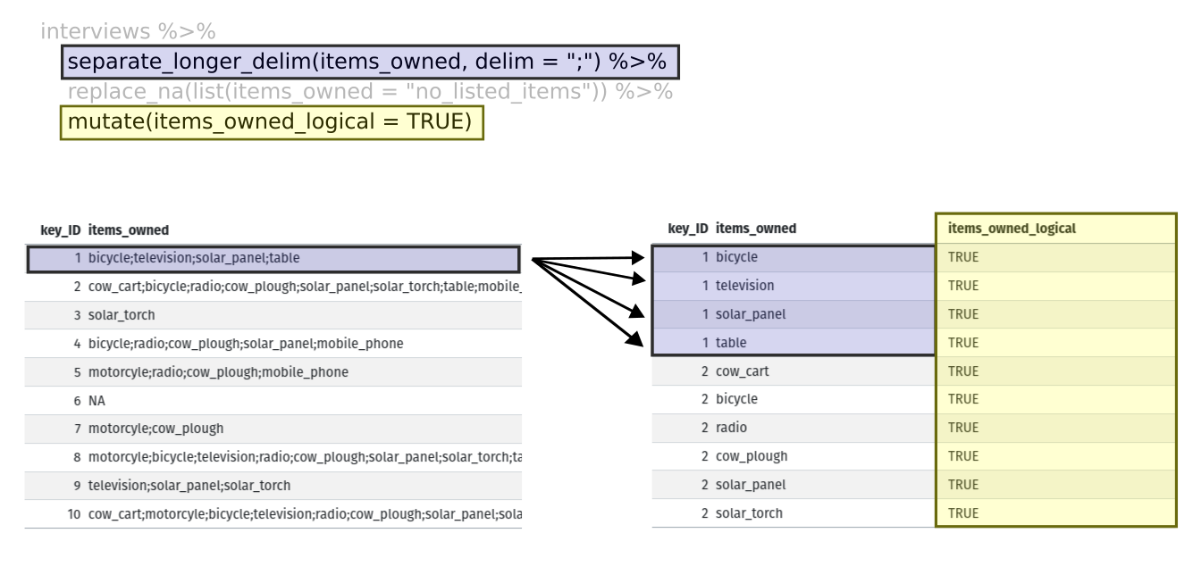
Then we will actually need to make our data frame longer, because we
have multiple items in a single cell. We will use a new function,
separate_longer_delim(), from the
tidyr package to separate the values of
items_owned based on the presence of semi-colons
(;). The values of this variable were multiple items
separated by semi-colons, so this action creates a row for each item
listed in a household’s possession. Thus, we end up with a long format
version of the dataset, with multiple rows for each respondent. For
example, if a respondent has a television and a solar panel, that
respondent will now have two rows, one with “television” and the other
with “solar panel” in the items_owned column.
After this transformation, you may notice that the
items_owned column contains NA values. This is
because some of the respondents did not own any of the items in the
interviewer’s list. We can use the replace_na() function to
change these NA values to something more meaningful. The
replace_na() function expects for you to give it a
list() of columns that you would like to replace the
NA values in, and the value that you would like to replace
the NAs. This ends up looking like this:
Next, we create a new variable named
items_owned_logical, which has one value
(TRUE) for every row. This makes sense, since each item in
every row was owned by that household. We are constructing this variable
so that when we spread the items_owned across multiple
columns, we can fill the values of those columns with logical values
describing whether the household did (TRUE) or did not
(FALSE) own that particular item.
At this point, we can also count the number of items owned by each
household, which is equivalent to the number of rows per
key_ID. We can do this with a group_by() and
mutate() pipeline that works similar to
group_by() and summarize() discussed in the
previous episode but instead of creating a summary table, we will add
another column called number_items. We use the
n() function to count the number of rows within each group.
However, there is one difficulty we need to take into account, namely
those households that did not list any items. These households now have
"no_listed_items" under items_owned. We do not
want to count this as an item but instead show zero items. We can
accomplish this using dplyr’s
if_else() function that evaluates a condition and returns
one value if true and another if false. Here, if the
items_owned column is "no_listed_items", then
a 0 is returned, otherwise, the number of rows per group is returned
using n().
Lastly, we use pivot_wider() to switch from long format
to wide format. This creates a new column for each of the unique values
in the items_owned column, and fills those columns with the
values of items_owned_logical. We also declare that for
items that are missing, we want to fill those cells with the value of
FALSE instead of NA.
R
pivot_wider(names_from = items_owned,
            values_from = items_owned_logical,
            values_fill = list(items_owned_logical = FALSE))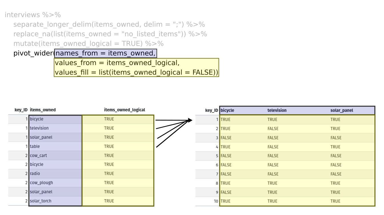
Combining the above steps, the chunk looks like this. Note that two
new columns are created within the same mutate() call.
R
interviews_items_owned <- interviews %>%
  separate_longer_delim(items_owned, delim = ";") %>%
  replace_na(list(items_owned = "no_listed_items")) %>%
  group_by(key_ID) %>%
  mutate(items_owned_logical = TRUE,
         number_items = if_else(items_owned == "no_listed_items", 0, n())) %>%
  pivot_wider(names_from = items_owned,
              values_from = items_owned_logical,
              values_fill = list(items_owned_logical = FALSE))
View the interviews_items_owned data frame. It should
have r nrow(interviews) rows (the same number of rows you
had originally), but extra columns for each item. How many columns were
added? Notice that there is no longer a column titled
items_owned. This is because there is a default parameter
in pivot_wider() that drops the original column. The values
that were in that column have now become columns named
television, solar_panel, table,
etc. You can use dim(interviews) and
dim(interviews_wide) to see how the number of columns has
changed between the two datasets.
This format of the data allows us to do interesting things, like make a table showing the number of respondents in each village who owned a particular item:
R
interviews_items_owned %>%
  filter(bicycle) %>%
  group_by(village) %>%
  count(bicycle)
OUTPUT
# A tibble: 3 × 3
# Groups:   village [3]
  village  bicycle     n
  <chr>    <lgl>   <int>
1 Chirodzo TRUE       17
2 God      TRUE       23
3 Ruaca    TRUE       20
Or below we calculate the average number of items from the list owned
by respondents in each village using the number_items
column we created to count the items listed by each household.
R
interviews_items_owned %>%
    group_by(village) %>%
    summarize(mean_items = mean(number_items))
OUTPUT
# A tibble: 3 × 2
  village  mean_items
  <chr>         <dbl>
1 Chirodzo       4.54
2 God            3.98
3 Ruaca          5.57
Exercise
We created interviews_items_owned by reshaping the data:
first longer and then wider. Replicate this process with the
months_lack_food column in the interviews
dataframe. Create a new dataframe with columns for each of the months
filled with logical vectors (TRUE or FALSE)
and a summary column called number_months_lack_food that
calculates the number of months each household reported a lack of
food.
Note that if the household did not lack food in the previous 12 months, the value input was “none”.
R
months_lack_food <- interviews %>%
  separate_longer_delim(months_lack_food, delim = ";") %>%
  group_by(key_ID) %>%
  mutate(months_lack_food_logical = TRUE,
         number_months_lack_food = if_else(months_lack_food == "none", 0, n())) %>%
  pivot_wider(names_from = months_lack_food,
              values_from = months_lack_food_logical,
              values_fill = list(months_lack_food_logical = FALSE))
Pivoting longer
The opposing situation could occur if we had been provided with data
in the form of interviews_wide, where the items owned are
column names, but we wish to treat them as values of an
items_owned variable instead.
In this situation we are gathering these columns turning them into a pair of new variables. One variable includes the column names as values, and the other variable contains the values in each cell previously associated with the column names. We will do this in two steps to make this process a bit clearer.
pivot_longer() takes four principal arguments:
- the data
- cols are the names of the columns we use to fill the a new values variable (or to drop).
- the names_to column variable we wish to create from the cols provided.
- the values_to column variable we wish to create and fill with values associated with the cols provided.
R
interviews_long <- interviews_items_owned %>%
  pivot_longer(cols = bicycle:car,
               names_to = "items_owned",
               values_to = "items_owned_logical")
View both interviews_long and
interviews_items_owned and compare their structure.
Exercise
We created some summary tables on interviews_items_owned
using count and summarise. We can create the
same tables on interviews_long, but this will require a
different process.
Make a table showing the number of respondents in each village who
owned a particular item, and include all items. The difference between
this format and the wide format is that you can now count
all the items using the items_owned variable.
R
interviews_long %>%
  filter(items_owned_logical) %>%
  group_by(village) %>%
  count(items_owned)
OUTPUT
# A tibble: 47 × 3
# Groups:   village [3]
   village  items_owned         n
   <chr>    <chr>           <int>
 1 Chirodzo bicycle            17
 2 Chirodzo computer            2
 3 Chirodzo cow_cart            6
 4 Chirodzo cow_plough         20
 5 Chirodzo electricity         1
 6 Chirodzo fridge              1
 7 Chirodzo lorry               1
 8 Chirodzo mobile_phone       25
 9 Chirodzo motorcyle          13
10 Chirodzo no_listed_items     3
# ℹ 37 more rows
Applying what we learned to clean our data
Now we have simultaneously learned about pivot_longer()
and pivot_wider(), and fixed a problem in the way our data
is structured. In this dataset, we have another column that stores
multiple values in a single cell. Some of the cells in the
months_lack_food column contain multiple months which, as
before, are separated by semi-colons (;).
To create a data frame where each of the columns contain only one
value per cell, we can repeat the steps we applied to
items_owned and apply them to
months_lack_food. Since we will be using this data frame
for the next episode, we will call it
interviews_plotting.
R
## Plotting data ##
interviews_plotting <- interviews %>%
  ## pivot wider by items_owned
  separate_longer_delim(items_owned, delim = ";") %>%
  replace_na(list(items_owned = "no_listed_items")) %>%
  ## Use of grouped mutate to find number of rows
  group_by(key_ID) %>%
  mutate(items_owned_logical = TRUE,
         number_items = if_else(items_owned == "no_listed_items", 0, n())) %>%
  pivot_wider(names_from = items_owned,
              values_from = items_owned_logical,
              values_fill = list(items_owned_logical = FALSE)) %>%
  ## pivot wider by months_lack_food
  separate_longer_delim(months_lack_food, delim = ";") %>%
  mutate(months_lack_food_logical = TRUE,
         number_months_lack_food = if_else(months_lack_food == "none", 0, n())) %>%
  pivot_wider(names_from = months_lack_food,
              values_from = months_lack_food_logical,
              values_fill = list(months_lack_food_logical = FALSE))
Exporting data
Now that you have learned how to use
dplyr and
tidyr to wrangle your raw data, you may
want to export these new datasets to share them with your collaborators
or for archival purposes.
Similar to the read_csv() function used for reading CSV
files into R, there is a write_csv() function that
generates CSV files from data frames.
Before using write_csv(), we are going to create a new
folder, data_output, in our working directory that will
store this generated dataset. We don’t want to write generated datasets
in the same directory as our raw data. It’s good practice to keep them
separate. The data folder should only contain the raw,
unaltered data, and should be left alone to make sure we don’t delete or
modify it. In contrast, our script will generate the contents of the
data_output directory, so even if the files it contains are
deleted, we can always re-generate them.
In preparation for our next lesson on plotting, we created a version
of the dataset where each of the columns includes only one data value.
Now we can save this data frame to our data_output
directory.
R
write_csv(interviews_plotting, file = "data_output/interviews_plotting.csv")Key Points
- Use the
tidyrpackage to change the layout of data frames. - Use
pivot_wider()to go from long to wide format. - Use
pivot_longer()to go from wide to long format.