Capstone Challenge
Last updated on 2024-03-12 | Edit this page
Overview
Questions
- How can we automatically count bacterial colonies with image analysis?
Objectives
- Bring together everything you’ve learnt so far to count bacterial colonies in 3 images.
In this episode, we will provide a final challenge for you to attempt, based on all the skills you have acquired so far. This challenge will be related to the shape of objects in images (morphometrics).
Morphometrics: Bacteria Colony Counting
As mentioned in the workshop introduction, your morphometric challenge is to determine how many bacteria colonies are in each of these images:
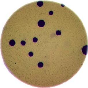
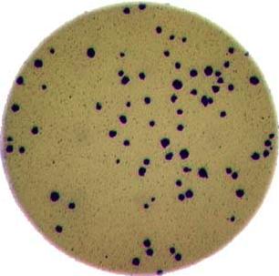
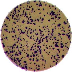
The image files can be found at data/colonies-01.tif,
data/colonies-02.tif, and
data/colonies-03.tif.
Morphometrics for bacterial colonies
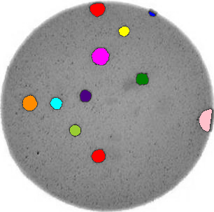
Write a Python program that uses scikit-image to count the number of bacteria colonies in each image, and for each, produce a new image that highlights the colonies. The image should look similar to this one:
Additionally, print out the number of colonies for each image.
Use what you have learnt about histograms, thresholding and connected component analysis. Try to put your code into a re-usable function, so that it can be applied conveniently to any image file.
First, let’s work through the process for one image:
PYTHON
import imageio.v3 as iio
import ipympl
import matplotlib.pyplot as plt
import numpy as np
import skimage as ski

%matplotlib widget

bacteria_image = iio.imread(uri="data/colonies-01.tif")

# display the image
fig, ax = plt.subplots()
ax.imshow(bacteria_image)
Next, we need to threshold the image to create a mask that covers only the dark bacterial colonies. This is easier using a grayscale image, so we convert it here:
PYTHON
gray_bacteria = ski.color.rgb2gray(bacteria_image)

# display the gray image
fig, ax = plt.subplots()
ax.imshow(gray_bacteria, cmap="gray")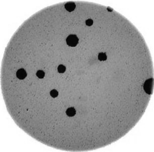
Next, we blur the image and create a histogram:
PYTHON
blurred_image = ski.filters.gaussian(gray_bacteria, sigma=1.0)
histogram, bin_edges = np.histogram(blurred_image, bins=256, range=(0.0, 1.0))
fig, ax = plt.subplots()
ax.plot(bin_edges[0:-1], histogram)
ax.set_title("Graylevel histogram")
ax.set_xlabel("gray value")
ax.set_ylabel("pixel count")
ax.set_xlim(0, 1.0)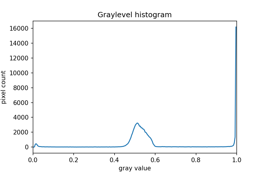
In this histogram, we see three peaks - the left one (i.e. the darkest pixels) is our colonies, the central peak is the yellow/brown culture medium in the dish, and the right one (i.e. the brightest pixels) is the white image background. Therefore, we choose a threshold that selects the small left peak:
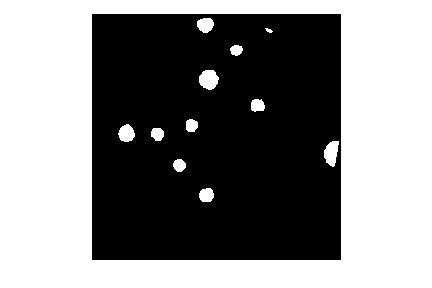
This mask shows us where the colonies are in the image - but how can we count how many there are? This requires connected component analysis:
Finally, we create the summary image of the coloured colonies on top of the grayscale image:
PYTHON
# color each of the colonies a different color
colored_label_image = ski.color.label2rgb(labeled_image, bg_label=0)
# give our grayscale image rgb channels, so we can add the colored colonies
summary_image = ski.color.gray2rgb(gray_bacteria)
summary_image[mask] = colored_label_image[mask]

# plot overlay
fig, ax = plt.subplots()
ax.imshow(summary_image)
Now that we’ve completed the task for one image, we need to repeat this for the remaining two images. This is a good point to collect the lines above into a re-usable function:
PYTHON
def count_colonies(image_filename):
    bacteria_image = iio.imread(image_filename)
    gray_bacteria = ski.color.rgb2gray(bacteria_image)
    blurred_image = ski.filters.gaussian(gray_bacteria, sigma=1.0)
    mask = blurred_image < 0.2
    labeled_image, count = ski.measure.label(mask, return_num=True)
    print(f"There are {count} colonies in {image_filename}")

    colored_label_image = ski.color.label2rgb(labeled_image, bg_label=0)
    summary_image = ski.color.gray2rgb(gray_bacteria)
    summary_image[mask] = colored_label_image[mask]
    fig, ax = plt.subplots()
    ax.imshow(summary_image)
Now we can do this analysis on all the images via a for loop:
PYTHON
for image_filename in ["data/colonies-01.tif", "data/colonies-02.tif", "data/colonies-03.tif"]:
    count_colonies(image_filename=image_filename)
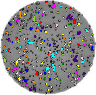
You’ll notice that for the images with more colonies, the results aren’t perfect. For example, some small colonies are missing, and there are likely some small black spots being labelled incorrectly as colonies. You could expand this solution to, for example, use an automatically determined threshold for each image, which may fit each better. Also, you could filter out colonies below a certain size (as we did in the Connected Component Analysis episode). You’ll also see that some touching colonies are merged into one big colony. This could be fixed with more complicated segmentation methods (outside of the scope of this lesson) like watershed.
Colony counting with minimum size and automated threshold (optional, not included in timing)
Modify your function from the previous exercise for colony counting to (i) exclude objects smaller than a specified size and (ii) use an automated thresholding approach, e.g. Otsu, to mask the colonies.
Here is a modified function with the requested features. Note when calculating the Otsu threshold we don’t include the very bright pixels outside the dish.
PYTHON
def count_colonies_enhanced(image_filename, sigma=1.0, min_colony_size=10, connectivity=2):

    bacteria_image = iio.imread(image_filename)
    gray_bacteria = ski.color.rgb2gray(bacteria_image)
    blurred_image = ski.filters.gaussian(gray_bacteria, sigma=sigma)

    # create mask excluding the very bright pixels outside the dish
    # we dont want to include these when calculating the automated threshold
    mask = blurred_image < 0.90
    # calculate an automated threshold value within the dish using the Otsu method
    t = ski.filters.threshold_otsu(blurred_image[mask])
    # update mask to select pixels both within the dish and less than t
    mask = np.logical_and(mask, blurred_image < t)
    # remove objects smaller than specified area
    mask = ski.morphology.remove_small_objects(mask, min_size=min_colony_size)

    labeled_image, count = ski.measure.label(mask, return_num=True)
    print(f"There are {count} colonies in {image_filename}")
    colored_label_image = ski.color.label2rgb(labeled_image, bg_label=0)
    summary_image = ski.color.gray2rgb(gray_bacteria)
    summary_image[mask] = colored_label_image[mask]
    fig, ax = plt.subplots()
    ax.imshow(summary_image)
Key Points
- Using thresholding, connected component analysis and other tools we can automatically segment images of bacterial colonies.
- These methods are useful for many scientific problems, especially those involving morphometrics.