Making the Isochrone DataFrame

Calculating Isochrone

In fact, we can use MESA Isochrones & Stellar Tracks (MIST) to compute it for us. Using the MIST Version 1.2 web interface, we computed an isochrone with the following parameters:

• Rotation initial v/v_crit = 0.4
• Single age, linear scale = 12e9
• Composition [Fe/H] = -1.35
• Synthetic Photometry, PanStarrs
• Extinction av = 0

The following cell downloads the results:

PYTHON

download('https://github.com/AllenDowney/AstronomicalData/raw/main/' +
         'data/MIST_iso_5fd2532653c27.iso.cmd')

To read this file we will download a Python module from this repository.

PYTHON

download('https://github.com/jieunchoi/MIST_codes/raw/master/scripts/' +
         'read_mist_models.py')

Now we can read the file:

PYTHON

import read_mist_models

filename = 'MIST_iso_5fd2532653c27.iso.cmd'
iso = read_mist_models.ISOCMD(filename)

OUTPUT

Reading in: MIST_iso_5fd2532653c27.iso.cmd

The result is an ISOCMD object.

PYTHON

type(iso)

OUTPUT

read_mist_models.ISOCMD

It contains a list of arrays, one for each isochrone.

PYTHON

type(iso.isocmds)

OUTPUT

list

We only got one isochrone.

PYTHON

len(iso.isocmds)

OUTPUT

1

So we can select it like this:

PYTHON

iso_array = iso.isocmds[0]

It is a NumPy array:

PYTHON

type(iso_array)

OUTPUT

numpy.ndarray

But it is an unusual NumPy array, because it contains names for the columns.

PYTHON

iso_array.dtype

OUTPUT

dtype([('EEP', '<i4'), ('isochrone_age_yr', '<f8'), ('initial_mass', '<f8'), ('star_mass', '<f8'), ('log_Teff', '<f8'), ('log_g', '<f8'), ('log_L', '<f8'), ('[Fe/H]_init', '<f8'), ('[Fe/H]', '<f8'), ('PS_g', '<f8'), ('PS_r', '<f8'), ('PS_i', '<f8'), ('PS_z', '<f8'), ('PS_y', '<f8'), ('PS_w', '<f8'), ('PS_open', '<f8'), ('phase', '<f8')])

Which means we can select columns using the bracket operator:

PYTHON

iso_array['phase']

OUTPUT

array([0., 0., 0., ..., 6., 6., 6.])

We can use phase to select the part of the isochrone for stars in the main sequence and red giant phases.

PYTHON

phase_mask = (iso_array['phase'] >= 0) & (iso_array['phase'] < 3)
phase_mask.sum()

OUTPUT

354

PYTHON

main_sequence = iso_array[phase_mask]
len(main_sequence)

OUTPUT

354

The other two columns we will use are PS_g and PS_i, which contain simulated photometry data for stars with the given age and metallicity, based on a model of the Pan-STARRS sensors.

We will use these columns to superimpose the isochrone on the color-magnitude diagram, but first we have to use a distance modulus to scale the isochrone based on the estimated distance of GD-1.

We can use the Distance object from Astropy to compute the distance modulus.

PYTHON

import astropy.coordinates as coord
import astropy.units as u

distance = 7.8 * u.kpc
distmod = coord.Distance(distance).distmod.value
distmod

OUTPUT

14.4604730134524

Now we can compute the scaled magnitude and color of the isochrone.

PYTHON

mag_g = main_sequence['PS_g'] + distmod
color_g_i = main_sequence['PS_g'] - main_sequence['PS_i']

Now we can plot it on the color-magnitude diagram like this.

PYTHON

plot_cmd(candidate_df)
plt.plot(color_g_i, mag_g);

OUTPUT

<Figure size 432x288 with 1 Axes>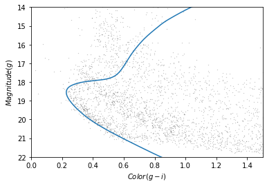

The theoretical isochrone passes through the overdense region where we expect to find stars in GD-1.

We will save this result so we can reload it later without repeating the steps in this section.

So we can save the data in an HDF5 file, we will put it in a Pandas DataFrame first:

PYTHON

import pandas as pd

iso_df = pd.DataFrame()
iso_df['mag_g'] = mag_g
iso_df['color_g_i'] = color_g_i

iso_df.head()

OUTPUT

       mag_g  color_g_i
0  28.294743   2.195021
1  28.189718   2.166076
2  28.051761   2.129312
3  27.916194   2.093721
4  27.780024   2.058585

And then save it.

PYTHON

filename = 'gd1_isochrone.hdf5'
iso_df.to_hdf(filename, 'iso_df')