Content from Introducing Databases and SQL

---

Last updated on 2023-04-21 | Edit this page

Overview

Questions

• What is a relational database and why should I use it?
• What is SQL?

Objectives

• Describe why relational databases are useful.
• Create and populate a database from a text file.
• Define SQLite data types.

Setup

Note: this should have been done by participants before the start of the workshop.

We use DB Browser for SQLite and the Portal Project dataset throughout this lesson. See Setup for instructions on how to download the data, and also how to install DB Browser for SQLite.

Motivation

---

To start, let’s orient ourselves in our project workflow. Previously, we used Excel and OpenRefine to go from messy, human created data to cleaned, computer-readable data. Now we’re going to move to the next piece of the data workflow, using the computer to read in our data, and then use it for analysis and visualization.

What is SQL?

SQL stands for Structured Query Language. SQL allows us to interact with relational databases through queries. These queries can allow you to perform a number of actions such as: insert, select, update and delete information in a database.

Dataset Description

The data we will be using is a time-series for a small mammal community in southern Arizona. This is part of a project studying the effects of rodents and ants on the plant community that has been running for almost 40 years. The rodents are sampled on a series of 24 plots, with different experimental manipulations controlling which rodents are allowed to access which plots.

This is a real dataset that has been used in over 100 publications. We’ve simplified it for the workshop, but you can download the full dataset and work with it using exactly the same tools we’ll learn about today.

Questions

Let’s look at some of the cleaned spreadsheets you downloaded during Setup to complete this challenge. You’ll need the following three files:

• surveys.csv
• species.csv
• plots.csv

Challenge

Open each of these csv files and explore them. What information is contained in each file? Specifically, if I had the following research questions:

• How has the hindfoot length and weight of Dipodomys species changed over time?
• What is the average weight of each species, per year?
• What information can I learn about Dipodomys species in the 2000s, over time?

What would I need to answer these questions? Which files have the data I need? What operations would I need to perform if I were doing these analyses by hand?

Goals

In order to answer the questions described above, we’ll need to do the following basic data operations:

• select subsets of the data (rows and columns)
• group subsets of data
• do math and other calculations
• combine data across spreadsheets

In addition, we don’t want to do this manually! Instead of searching for the right pieces of data ourselves, or clicking between spreadsheets, or manually sorting columns, we want to make the computer do the work.

In particular, we want to use a tool where it’s easy to repeat our analysis in case our data changes. We also want to do all this searching without actually modifying our source data.

Putting our data into a relational database and using SQL will help us achieve these goals.

Definition:Relational Database

A relational database stores data in relations made up of records with fields. The relations are usually represented as tables; each record is usually shown as a row, and the fields as columns. In most cases, each record will have a unique identifier, called a key, which is stored as one of its fields. Records may also contain keys that refer to records in other tables, which enables us to combine information from two or more sources.

Databases

---

Why use relational databases

Using a relational database serves several purposes.

• It keeps your data separate from your analysis.
  • This means there’s no risk of accidentally changing data when you analyze it.
  • If we get new data we can rerun the query.
• It’s fast, even for large amounts of data.
• It improves quality control of data entry (type constraints and use of forms in MS Access, Filemaker, Oracle Application Express etc.)
• The concepts of relational database querying are core to understanding how to do similar things using programming languages such as R or Python.

Database Management Systems

There are different database management systems to work with relational databases such as SQLite, MySQL, PostgreSQL, MSSQL Server, and many more. Each of them differ mainly based on their scalability, but they all share the same core principles of relational databases. In this lesson, we use SQLite to introduce you to SQL and data retrieval from a relational database.

Relational databases

Let’s look at a pre-existing database, the portal_mammals.sqlite file from the Portal Project dataset that we downloaded during Setup. Click on the “Open Database” button, select the portal_mammals.sqlite file, and click “Open” to open the database.

You can see the tables in the database by looking at the left hand side of the screen under Database Structure tab. Here you will see a list under “Tables.” Each item listed here corresponds to one of the csv files we were exploring earlier. To see the contents of any table, right-click on it, and then click the “Browse Table” from the menu, or select the “Browse Data” tab next to the “Database Structure” tab and select the wanted table from the dropdown named “Table”. This will give us a view that we’re used to - a copy of the table. Hopefully this helps to show that a database is, in some sense, just a collection of tables, where there’s some value in the tables that allows them to be connected to each other (the “related” part of “relational database”).

The “Database Structure” tab also provides some metadata about each table. If you click on the down arrow next to a table name, you will see information about the columns, which in databases are referred to as “fields,” and their assigned data types. (The rows of a database table are called records.) Each field contains one variety or type of data, often numbers or text. You can see in the surveys table that most fields contain numbers (BIGINT, or big integer, and FLOAT, or floating point numbers/decimals) while the species table is entirely made up of text fields.

The “Execute SQL” tab is blank now - this is where we’ll be typing our queries to retrieve information from the database tables.

To summarize:

• Relational databases store data in tables with fields (columns) and records (rows)
• Data in tables has types, and all values in a field have the same type (list of data types)
• Queries let us look up data or make calculations based on columns

Database Design

• Every row-column combination contains a single atomic value, i.e., not containing parts we might want to work with separately.
• One field per type of information
• No redundant information
  • Split into separate tables with one table per class of information
  • Needs an identifier in common between tables – shared column - to reconnect (known as a foreign key).

Import

Before we get started with writing our own queries, we’ll create our own database. We’ll be creating this database from the three csv files we downloaded earlier. Close the currently open database (File > Close Database) and then follow these instructions:

1. Start a New Database

• Click the New Database button
• Give a name and click Save to create the database in the opened folder
• In the “Edit table definition” window that pops up, click cancel as we will be importing tables, not creating them from scratch

2. Select File >> Import >> Table from CSV file…
3. Choose surveys.csv from the data folder we downloaded and click Open.
4. Give the table a name that matches the file name (surveys), or use the default
5. If the first row has column headings, be sure to check the box next to “Column names in first line”.
6. Be sure the field separator and quotation options are correct. If you’re not sure which options are correct, test some of the options until the preview at the bottom of the window looks right.
7. Press OK, you should subsequently get a message that the table was imported.
8. Back on the Database Structure tab, you should now see the table listed. Right click on the table name and choose Modify Table, or click on the Modify Table button just under the tabs and above the table list.
9. Click Save if asked to save all pending changes.
10. In the center panel of the window that appears, set the data types for each field using the suggestions in the table below (this includes fields from the plots and species tables also).
11. Finally, click OK one more time to confirm the operation. Then click the Write Changes button to save the database.

Field	Data Type	Motivation	Table(s)
day	INTEGER	Having data as numeric allows for meaningful arithmetic and comparisons	surveys
genus	TEXT	Field contains text data	species
hindfoot_length	REAL	Field contains measured numeric data	surveys
month	INTEGER	Having data as numeric allows for meaningful arithmetic and comparisons	surveys
plot_id	INTEGER	Field contains numeric data	plots, surveys
plot_type	TEXT	Field contains text data	plots
record_id	INTEGER	Field contains numeric data	surveys
sex	TEXT	Field contains text data	surveys
species_id	TEXT	Field contains text data	species, surveys
species	TEXT	Field contains text data	species
taxa	TEXT	Field contains text data	species
weight	REAL	Field contains measured numerical data	surveys
year	INTEGER	Allows for meaningful arithmetic and comparisons	surveys

Challenge

• Import the plots and species tables

You can also use this same approach to append new fields to an existing table.

Adding fields to existing tables

1. Go to the “Database Structure” tab, right click on the table you’d like to add data to, and choose Modify Table, or click on the Modify Table just under the tabs and above the table.
2. Click the Add Field button to add a new field and assign it a data type.

Data types

Data type	Description
CHARACTER(n)	Character string. Fixed-length n
VARCHAR(n) or CHARACTER VARYING(n)	Character string. Variable length. Maximum length n
BINARY(n)	Binary string. Fixed-length n
BOOLEAN	Stores TRUE or FALSE values
VARBINARY(n) or BINARY VARYING(n)	Binary string. Variable length. Maximum length n
INTEGER(p)	Integer numerical (no decimal).
SMALLINT	Integer numerical (no decimal).
INTEGER	Integer numerical (no decimal).
BIGINT	Integer numerical (no decimal).
DECIMAL(p,s)	Exact numerical, precision p, scale s.
NUMERIC(p,s)	Exact numerical, precision p, scale s. (Same as DECIMAL)
FLOAT(p)	Approximate numerical, mantissa precision p. A floating number in base 10 exponential notation.
REAL	Approximate numerical
FLOAT	Approximate numerical
DOUBLE PRECISION	Approximate numerical
DATE	Stores year, month, and day values
TIME	Stores hour, minute, and second values
TIMESTAMP	Stores year, month, day, hour, minute, and second values
INTERVAL	Composed of a number of integer fields, representing a period of time, depending on the type of interval
ARRAY	A set-length and ordered collection of elements
MULTISET	A variable-length and unordered collection of elements
XML	Stores XML data

SQL Data Type Quick Reference

Different databases offer different choices for the data type definition.

The following table shows some of the common names of data types between the various database platforms:

Data type	Access	SQLServer	Oracle	MySQL	PostgreSQL
boolean	Yes/No	Bit	Byte	N/A	Boolean
integer	Number (integer)	Int	Number	Int / Integer	Int / Integer
float	Number (single)	Float / Real	Number	Float	Numeric
currency	Currency	Money	N/A	N/A	Money
string (fixed)	N/A	Char	Char	Char	Char
string (variable)	Text (<256) / Memo (65k+)	Varchar	Varchar2	Varchar	Varchar
binary object OLE Object Memo Binary (fixed up to 8K)	Varbinary (<8K)	Image (<2GB) Long	Raw Blob	Text Binary	Varbinary

Key Points

• SQL allows us to select and group subsets of data, do math and other calculations, and combine data.
• A relational database is made up of tables which are related to each other by shared keys.
• Different database management systems (DBMS) use slightly different vocabulary, but they are all based on the same ideas.

Content from Accessing Data With Queries

---

Last updated on 2023-04-21 | Edit this page

Overview

Questions

• How do I write a basic query in SQL?

Objectives

• Write and build queries.
• Filter data given various criteria.
• Sort the results of a query.

Writing my first query

---

Let’s start by using the surveys table. Here we have data on every individual that was captured at the site, including when they were captured, what plot they were captured on, their species ID, sex and weight in grams.

Let’s write an SQL query that selects all of the columns in the surveys table. SQL queries can be written in the box located under the “Execute SQL” tab. Click on the right arrow above the query box to execute the query. (You can also use the keyboard shortcut “Cmd-Enter” on a Mac or “Ctrl-Enter” on a Windows machine to execute a query.) The results are displayed in the box below your query. If you want to display all of the columns in a table, use the wildcard *.

SQL

SELECT *
FROM surveys;

We have capitalized the words SELECT and FROM because they are SQL keywords. SQL is case insensitive, but it helps for readability, and is good style.

If we want to select a single column, we can type the column name instead of the wildcard *.

SQL

SELECT year
FROM surveys;

If we want more information, we can add more columns to the list of fields, right after SELECT:

SQL

SELECT year, month, day
FROM surveys;

Limiting results

Sometimes you don’t want to see all the results, you just want to get a sense of what’s being returned. In that case, you can use a LIMIT clause. In particular, you would want to do this if you were working with large databases.

SQL

SELECT *
FROM surveys
LIMIT 10;

Unique values

If we want only the unique values so that we can quickly see what species have been sampled we use DISTINCT

SQL

SELECT DISTINCT species_id
FROM surveys;

If we select more than one column, then the distinct pairs of values are returned

SQL

SELECT DISTINCT year, species_id
FROM surveys;

Calculated values

We can also do calculations with the values in a query. For example, if we wanted to look at the mass of each individual on different dates, but we needed it in kg instead of g we would use

SQL

SELECT year, month, day, weight/1000
FROM surveys;

When we run the query, the expression weight / 1000 is evaluated for each row and appended to that row, in a new column. If we used the INTEGER data type for the weight field then integer division would have been done, to obtain the correct results in that case divide by 1000.0. Expressions can use any fields, any arithmetic operators (+, -, *, and /) and a variety of built-in functions. For example, we could round the values to make them easier to read.

SQL

SELECT plot_id, species_id, sex, weight, ROUND(weight / 1000, 2)
FROM surveys;

Challenge

• Write a query that returns the year, month, day, species_id and weight in mg.

Show me the solution

SQL

SELECT day, month, year, species_id, weight * 1000
FROM surveys;

Filtering

---

Databases can also filter data – selecting only the data meeting certain criteria. For example, let’s say we only want data for the species Dipodomys merriami, which has a species code of DM. We need to add a WHERE clause to our query:

SQL

SELECT *
FROM surveys
WHERE species_id='DM';

We can do the same thing with numbers. Here, we only want the data since 2000:

SQL

SELECT * FROM surveys
WHERE year >= 2000;

If we used the TEXT data type for the year, the WHERE clause should be year >= '2000'.

We can use more sophisticated conditions by combining tests with AND and OR. For example, suppose we want the data on Dipodomys merriami starting in the year 2000:

SQL

SELECT *
FROM surveys
WHERE (year >= 2000) AND (species_id = 'DM');

Note that the parentheses are not needed, but again, they help with readability. They also ensure that the computer combines AND and OR in the way that we intend.

If we wanted to get data for any of the Dipodomys species, which have species codes DM, DO, and DS, we could combine the tests using OR:

SQL

SELECT *
FROM surveys
WHERE (species_id = 'DM') OR (species_id = 'DO') OR (species_id = 'DS');

Challenge

• Produce a table listing the data for all individuals in Plot 1 that weighed more than 75 grams, telling us the date, species id code, and weight (in kg).

Show me the solution

SQL

SELECT day, month, year, species_id, weight / 1000
FROM surveys
WHERE (plot_id = 1) AND (weight > 75);

Building more complex queries

---

Now, let’s combine the above queries to get data for the 3 Dipodomys species from the year 2000 on. This time, let’s use IN as one way to make the query easier to understand. It is equivalent to saying WHERE (species_id = 'DM') OR (species_id = 'DO') OR (species_id = 'DS'), but reads more neatly:

SQL

SELECT *
FROM surveys
WHERE (year >= 2000) AND (species_id IN ('DM', 'DO', 'DS'));

We started with something simple, then added more clauses one by one, testing their effects as we went along. For complex queries, this is a good strategy, to make sure you are getting what you want. Sometimes it might help to take a subset of the data that you can easily see in a temporary database to practice your queries on before working on a larger or more complicated database.

When the queries become more complex, it can be useful to add comments. In SQL, comments are started by --, and end at the end of the line. For example, a commented version of the above query can be written as:

SQL

-- Get post 2000 data on Dipodomys' species
-- These are in the surveys table, and we are interested in all columns
SELECT * FROM surveys
-- Sampling year is in the column `year`, and we want to include 2000
WHERE (year >= 2000)
-- Dipodomys' species have the `species_id` DM, DO, and DS
AND (species_id IN ('DM', 'DO', 'DS'));

Although SQL queries often read like plain English, it is always useful to add comments; this is especially true of more complex queries.

Sorting

---

We can also sort the results of our queries by using ORDER BY. For simplicity, let’s go back to the species table and alphabetize it by taxa.

First, let’s look at what’s in the species table. It’s a table of the species_id and the full genus, species and taxa information for each species_id. Having this in a separate table is nice, because we didn’t need to include all this information in our main surveys table.

SQL

SELECT *
FROM species;

Now let’s order it by taxa.

SQL

SELECT *
FROM species
ORDER BY taxa ASC;

The keyword ASC tells us to order it in ascending order. We could alternately use DESC to get descending order.

SQL

SELECT *
FROM species
ORDER BY taxa DESC;

ASC is the default.

We can also sort on several fields at once. To truly be alphabetical, we might want to order by genus then species.

SQL

SELECT *
FROM species
ORDER BY genus ASC, species ASC;

Challenge

• Write a query that returns year, species_id, and weight in kg from the surveys table, sorted with the largest weights at the top.

Show me the solution

SQL

SELECT year, species_id, weight / 1000
FROM surveys
ORDER BY weight DESC;

Order of execution

---

Another note for ordering. We don’t actually have to display a column to sort by it. For example, let’s say we want to order the birds by their species ID, but we only want to see genus and species.

SQL

SELECT genus, species
FROM species
WHERE taxa = 'Bird'
ORDER BY species_id ASC;

We can do this because sorting occurs earlier in the computational pipeline than field selection.

The computer is basically doing this:

1. Filtering rows according to WHERE
2. Sorting results according to ORDER BY
3. Displaying requested columns or expressions.

Clauses are written in a fixed order: SELECT, FROM, WHERE, then ORDER BY.

Multiple statements

It is possible to write a query as a single line, but for readability, we recommend to put each clause on its own line. The standard way to separate a whole SQL statement is with a semicolon. This allows more than one SQL statement to be executed together.

Challenge

• Let’s try to combine what we’ve learned so far in a single query. Using the surveys table, write a query to display the three date fields, species_id, and weight in kilograms (rounded to two decimal places), for individuals captured in 1999, ordered alphabetically by the species_id.
• Write the query as a single line, then put each clause on its own line, and see how more legible the query becomes!

Show me the solution

SQL

SELECT year, month, day, species_id, ROUND(weight / 1000, 2)
FROM surveys
WHERE year = 1999
ORDER BY species_id;

Key Points

• It is useful to apply conventions when writing SQL queries to aid readability.
• Use logical connectors such as AND or OR to create more complex queries.
• Calculations using mathematical symbols can also be performed on SQL queries.
• Adding comments in SQL helps keep complex queries understandable.

Content from Aggregating and Grouping Data

---

Last updated on 2023-04-21 | Edit this page

Overview

Questions

• How can I summarize my data by aggregating, filtering, or ordering query results?
• How can I make sure column names from my queries make sense and aren’t too long?

Objectives

• Apply aggregation functions to group records together.
• Filter and order results of a query based on aggregate functions.
• Employ aliases to assign new names to items in a query.
• Save a query to make a new table.
• Apply filters to find missing values in SQL.

COUNT and GROUP BY

---

Aggregation allows us to combine results by grouping records based on value. It is also useful for calculating combined values in groups.

Let’s go to the surveys table and find out how many individuals there are. Using the wildcard * counts the number of records (rows):

SQL

SELECT COUNT(*)
FROM surveys;

We can also find out how much all of those individuals weigh:

SQL

SELECT COUNT(*), SUM(weight)
FROM surveys;

We can output this value in kilograms (dividing the value by 1000.00), then rounding to 3 decimal places: (Notice the divisor has numbers after the decimal point, which forces the answer to have a decimal fraction)

SQL

SELECT ROUND(SUM(weight)/1000.00, 3)
FROM surveys;

There are many other aggregate functions included in SQL, for example: MAX, MIN, and AVG.

Challenge

Write a query that returns: the total weight, average weight, minimum and maximum weights for all animals caught over the duration of the survey. Can you modify it so that it outputs these values only for weights between 5 and 10?

Show me the solution

SQL

-- All animals
SELECT SUM(weight), AVG(weight), MIN(weight), MAX(weight)
FROM surveys;

-- Only weights between 5 and 10
SELECT SUM(weight), AVG(weight), MIN(weight), MAX(weight)
FROM surveys
WHERE (weight > 5) AND (weight < 10);

Now, let’s see how many individuals were counted in each species. We do this using a GROUP BY clause

SQL

SELECT species_id, COUNT(*)
FROM surveys
GROUP BY species_id;

GROUP BY tells SQL what field or fields we want to use to aggregate the data. If we want to group by multiple fields, we give GROUP BY a comma separated list.

Challenge

Write queries that return:

1. How many individuals were counted in each year in total
2. How many were counted each year, for each different species
3. The average weights of each species in each year

Can you get the answer to both 2 and 3 in a single query?

Solution of 1

SQL

SELECT year, COUNT(*)
FROM surveys
GROUP BY year;

Solution of 2 and 3

SQL

SELECT year, species_id, COUNT(*), AVG(weight)
FROM surveys
GROUP BY year, species_id;

Ordering Aggregated Results

---

We can order the results of our aggregation by a specific column, including the aggregated column. Let’s count the number of individuals of each species captured, ordered by the count:

SQL

SELECT species_id, COUNT(*)
FROM surveys
GROUP BY species_id
ORDER BY COUNT(species_id);

Aliases

---

As queries get more complex, the expressions we use can get long and unwieldy. To help make things clearer in the query and in its output, we can use aliases to assign new names to things in the query.

We can use aliases in column names using AS:

SQL

SELECT MAX(year) AS last_surveyed_year
FROM surveys;

The AS isn’t technically required, so you could do

SQL

SELECT MAX(year) last_surveyed_year
FROM surveys;

but using AS is much clearer so it is good style to include it.

We can not only alias column names, but also table names in the same way:

SQL

SELECT *
FROM surveys AS surv;

And again, the AS keyword is not required, so this works, too:

SQL

SELECT *
FROM surveys surv;

Aliasing table names can be helpful when working with queries that involve multiple tables; you will learn more about this later.

The HAVING keyword

---

In the previous episode, we have seen the keyword WHERE, allowing to filter the results according to some criteria. SQL offers a mechanism to filter the results based on aggregate functions, through the HAVING keyword.

For example, we can request to only return information about species with a count higher than 10:

SQL

SELECT species_id, COUNT(species_id)
FROM surveys
GROUP BY species_id
HAVING COUNT(species_id) > 10;

The HAVING keyword works exactly like the WHERE keyword, but uses aggregate functions instead of database fields to filter.

You can use the AS keyword to assign an alias to a column or table, and refer to that alias in the HAVING clause. For example, in the above query, we can call the COUNT(species_id) by another name, like occurrences. This can be written this way:

SQL

SELECT species_id, COUNT(species_id) AS occurrences
FROM surveys
GROUP BY species_id
HAVING occurrences > 10;

Note that in both queries, HAVING comes after GROUP BY. One way to think about this is: the data are retrieved (SELECT), which can be filtered (WHERE), then joined in groups (GROUP BY); finally, we can filter again based on some of these groups (HAVING).

Challenge

Write a query that returns, from the species table, the number of species in each taxa, only for the taxa with more than 10 species.

Show me the solution

SQL

SELECT taxa, COUNT(*) AS n
FROM species
GROUP BY taxa
HAVING n > 10;

Saving Queries for Future Use

---

It is not uncommon to repeat the same operation more than once, for example for monitoring or reporting purposes. SQL comes with a very powerful mechanism to do this by creating views. Views are a form of query that is saved in the database, and can be used to look at, filter, and even update information. One way to think of views is as a table, that can read, aggregate, and filter information from several places before showing it to you.

Creating a view from a query requires us to add CREATE VIEW viewname AS before the query itself. For example, imagine that our project only covers the data gathered during the summer (May - September) of 2000. That query would look like:

SQL

SELECT *
FROM surveys
WHERE year = 2000 AND (month > 4 AND month < 10);

But we don’t want to have to type that every time we want to ask a question about that particular subset of data. Hence, we can benefit from a view:

SQL

CREATE VIEW summer_2000 AS
SELECT *
FROM surveys
WHERE year = 2000 AND (month > 4 AND month < 10);

Using a view we will be able to access these results with a much shorter notation:

SQL

SELECT *
FROM summer_2000
WHERE species_id = 'PE';

What About NULL?

---

From the last example, there should only be five records. If you look at the weight column, it’s easy to see what the average weight would be. If we use SQL to find the average weight, SQL behaves like we would hope, ignoring the NULL values:

SQL

SELECT AVG(weight)
FROM summer_2000
WHERE species_id = 'PE';

But if we try to be extra clever, and find the average ourselves, we might get tripped up:

SQL

SELECT SUM(weight), COUNT(*), SUM(weight)/COUNT(*)
FROM summer_2000
WHERE species_id = 'PE';

Here the COUNT function includes all five records (even those with NULL values), but the SUM only includes the three records with data in the weight field, giving us an incorrect average. However, our strategy will work if we modify the COUNT function slightly:

SQL

SELECT SUM(weight), COUNT(weight), SUM(weight)/COUNT(weight)
FROM summer_2000
WHERE species_id = 'PE';

When we count the weight field specifically, SQL ignores the records with data missing in that field. So here is one example where NULLs can be tricky: COUNT(*) and COUNT(field) can return different values.

Another case is when we use a “negative” query. Let’s count all the non-female animals:

SQL

SELECT COUNT(*)
FROM summer_2000
WHERE sex != 'F';

Now let’s count all the non-male animals:

SQL

SELECT COUNT(*)
FROM summer_2000
WHERE sex != 'M';

But if we compare those two numbers with the total:

SQL

SELECT COUNT(*)
FROM summer_2000;

We’ll see that they don’t add up to the total! That’s because SQL doesn’t automatically include NULL values in a negative conditional statement. So if we are querying “not x”, then SQL divides our data into three categories: ‘x’, ‘not NULL, not x’ and NULL; then, returns the ‘not NULL, not x’ group. Sometimes this may be what we want - but sometimes we may want the missing values included as well! In that case, we’d need to change our query to:

SQL

SELECT COUNT(*)
FROM summer_2000
WHERE sex != 'M' OR sex IS NULL;

Key Points

• Use the GROUP BY keyword to aggregate data.
• Functions like MIN, MAX, AVG, SUM, COUNT, etc. operate on aggregated data.
• Aliases can help shorten long queries. To write clear and readable queries, use the AS keyword when creating aliases.
• Use the HAVING keyword to filter on aggregate properties.
• Use a VIEW to access the result of a query as though it was a new table.

Content from Combining Data With Joins

---

Last updated on 2023-06-30 | Edit this page

Overview

Questions

• How do I bring data together from separate tables?

Objectives

• Employ joins to combine data from two tables.
• Apply functions to manipulate individual values.
• Employ aliases to assign new names to tables and columns in a query.

Joins

---

To combine data from two tables we use an SQL JOIN clause, which comes after the FROM clause.

Database tables are used to organize and group data by common characteristics or principles.
Often, we need to combine elements from separate tables into a single tables or queries for analysis and visualization. A JOIN is a means for combining columns from multiple tables by using values common to each.

The JOIN keyword combined with ON is used to combine fields from separate tables.

A JOIN clause on its own will result in a cross product, where each row in the first table is paired with each row in the second table. Usually this is not what is desired when combining two tables with data that is related in some way.

For that, we need to tell the computer which columns provide the link between the two tables using the word ON. What we want is to join the data with the same species id.

SQL

SELECT *
FROM surveys
JOIN species
ON surveys.species_id = species.species_id;

ON is like WHERE. It filters things out according to a test condition. We use the table.colname format to tell the manager what column in which table we are referring to.

The output from using the JOIN clause will have columns from the first table plus the columns from the second table. For the above statement, the output will be a table that has the following column names:

record_id	month	day	year	plot_id	species_id	sex	hindfoot_length	weight	species_id	genus	species	taxa
…
96	8	20	1997	12	DM	M	36	41	DM	Dipodomys	merriami	Rodent
…

Alternatively, we can use the word USING, as a short-hand. USING only works on columns which share the same name. In this case we are telling the manager that we want to combine surveys with species and that the common column is species_id.

SQL

SELECT *
FROM surveys
JOIN species
USING (species_id);

The output will only have one species_id column

record_id	month	day	year	plot_id	species_id	sex	hindfoot_length	weight	genus	species	taxa
…
96	8	20	1997	12	DM	M	36	41	Dipodomys	merriami	Rodent
…

We often won’t want all of the fields from both tables, so anywhere we would have used a field name in a non-join query, we can use table.colname.

For example, what if we wanted information on when individuals of each species were captured, but instead of their species ID we wanted their actual species names.

SQL

SELECT surveys.year, surveys.month, surveys.day, species.genus, species.species
FROM surveys
JOIN species
ON surveys.species_id = species.species_id;

year	month	day	genus	species
…
1977	7	16	Neotoma	albigula
1977	7	16	Dipodomys	merriami
…

Many databases, including SQLite, also support a join through the WHERE clause of a query.
For example, you may see the query above written without an explicit JOIN.

SQL

SELECT surveys.year, surveys.month, surveys.day, species.genus, species.species
FROM surveys, species
WHERE surveys.species_id = species.species_id;

For the remainder of this lesson, we’ll stick with the explicit use of the JOIN keyword for joining tables in SQL.

Challenge:

• Write a query that returns the genus, the species name, and the weight of every individual captured at the site

Show me the solution

SQL

SELECT species.genus, species.species, surveys.weight
FROM surveys
JOIN species
ON surveys.species_id = species.species_id;

Different join types

We can count the number of records returned by our original join query.

SQL

SELECT COUNT(*)
FROM surveys
JOIN species
USING (species_id);

Notice that this number is smaller than the number of records present in the survey data.

SQL

SELECT COUNT(*) FROM surveys;

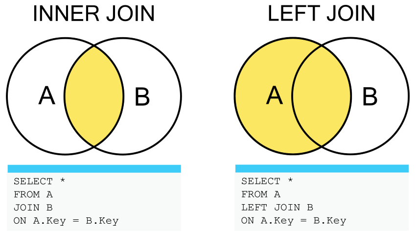
This is because, by default, SQL only returns records where the joining value is present in the joined columns of both tables (i.e. it takes the intersection of the two join columns). This joining behaviour is known as an INNER JOIN. In fact the JOIN keyword is simply shorthand for INNER JOIN and the two terms can be used interchangeably as they will produce the same result.

We can also tell the computer that we wish to keep all the records in the first table by using a LEFT OUTER JOIN clause, or LEFT JOIN for short. The difference between the two JOINs can be visualized like so:

Diagrams representing INNER JOIN and LEFT JOIN in SQLite

Challenge:

• Re-write the original query to keep all the entries present in the surveys table. How many records are returned by this query?

Show me the solution

SQL

SELECT * FROM surveys
LEFT JOIN species
USING (species_id);

Challenge:

• Count the number of records in the surveys table that have a NULL value in the species_id column.

Show me the solution

SQL

SELECT COUNT(*)
FROM surveys
WHERE species_id IS NULL;

Remember: In SQL a NULL value in one table can never be joined to a NULL value in a second table because NULL is not equal to anything, not even itself.

Combining joins with sorting and aggregation

Joins can be combined with sorting, filtering, and aggregation. So, if we wanted average mass of the individuals on each different type of treatment, we could do something like

SQL

SELECT plots.plot_type, AVG(surveys.weight)
FROM surveys
JOIN plots
ON surveys.plot_id = plots.plot_id
GROUP BY plots.plot_type;

Challenge:

• Write a query that returns the number of animals caught of each genus in each plot. Order the results by plot number (ascending) and by descending number of individuals in each plot.

Show me the solution

SQL

SELECT surveys.plot_id, species.genus, COUNT(*) AS number_indiv
FROM surveys
JOIN species
ON surveys.species_id = species.species_id
GROUP BY species.genus, surveys.plot_id
ORDER BY surveys.plot_id ASC, number_indiv DESC;

Challenge:

• Write a query that finds the average weight of each rodent species (i.e., only include species with Rodent in the taxa field).

Show me the solution

SQL

SELECT surveys.species_id, AVG(surveys.weight)
FROM surveys
JOIN species
ON surveys.species_id = species.species_id
WHERE species.taxa = 'Rodent'
GROUP BY surveys.species_id;

Functions COALESCE and NULLIF and more

---

SQL includes numerous functions for manipulating data. You’ve already seen some of these being used for aggregation (SUM and COUNT) but there are functions that operate on individual values as well. Probably the most important of these are COALESCE and NULLIF. COALESCE allows us to specify a value to use in place of NULL.

We can represent unknown sexes with 'U' instead of NULL:

SQL

SELECT species_id, sex, COALESCE(sex, 'U')
FROM surveys;

The lone “sex” column is only included in the query above to illustrate where COALESCE has changed values; this isn’t a usage requirement.

Challenge:

• Write a query that returns 30 instead of NULL for values in the hindfoot_length column.

Show me the solution

SQL

SELECT hindfoot_length, COALESCE(hindfoot_length, 30)
FROM surveys;

Challenge:

• Write a query that calculates the average hind-foot length of each species, assuming that unknown lengths are 30 (as above).

Show me the solution

SQL

SELECT species_id, AVG(COALESCE(hindfoot_length, 30))
FROM surveys
GROUP BY species_id;

COALESCE can be particularly useful in JOIN. When joining the species and surveys tables earlier, some results were excluded because the species_id was NULL in the surveys table. We can use COALESCE to include them again, re-writing the NULL to a valid joining value:

SQL

SELECT surveys.year, surveys.month, surveys.day, species.genus, species.species
FROM surveys
JOIN species
ON COALESCE(surveys.species_id, 'AB') = species.species_id;

Challenge:

• Write a query that returns the number of animals caught of each genus in each plot, assuming that unknown species are all of the genus “Rodent”.

Show me the solution

SQL

SELECT plot_id, COALESCE(genus, 'Rodent') AS genus2, COUNT(*)
FROM surveys 
LEFT JOIN species
ON surveys.species_id=species.species_id
GROUP BY plot_id, genus2;

The inverse of COALESCE is NULLIF. This returns NULL if the first argument is equal to the second argument. If the two are not equal, the first argument is returned. This is useful for “nulling out” specific values.

We can “null out” plot 7:

SQL

SELECT species_id, plot_id, NULLIF(plot_id, 7)
FROM surveys;

Some more functions which are common to SQL databases are listed in the table below:

Function	Description
ABS(n)	Returns the absolute (positive) value of the numeric expression n
COALESCE(x1, ..., xN)	Returns the first of its parameters that is not NULL
LENGTH(s)	Returns the length of the string expression s
LOWER(s)	Returns the string expression s converted to lowercase
NULLIF(x, y)	Returns NULL if x is equal to y, otherwise returns x
ROUND(n) or ROUND(n, x)	Returns the numeric expression n rounded to x digits after the decimal point (0 by default)
TRIM(s)	Returns the string expression s without leading and trailing whitespace characters
UPPER(s)	Returns the string expression s converted to uppercase

Finally, some useful functions which are particular to SQLite are listed in the table below:

Function	Description
RANDOM()	Returns a random integer between -9223372036854775808 and +9223372036854775807.
REPLACE(s, f, r)	Returns the string expression s in which every occurrence of f has been replaced with r
SUBSTR(s, x, y) or SUBSTR(s, x)	Returns the portion of the string expression s starting at the character position x (leftmost position is 1), y characters long (or to the end of s if y is omitted)

Challenge:

Write a query that returns genus names (no repeats), sorted from longest genus name down to shortest.

Show me the solution

SQL

SELECT DISTINCT genus
FROM species
ORDER BY LENGTH(genus) DESC;

As we saw before, aliases make things clearer, and are especially useful when joining tables.

SQL

SELECT surv.year AS yr, surv.month AS mo, surv.day AS day, sp.genus AS gen, sp.species AS sp
FROM surveys AS surv
JOIN species AS sp
ON surv.species_id = sp.species_id;

To practice we have some optional challenges for you.

Challenge (optional):

SQL queries help us ask specific questions which we want to answer about our data. The real skill with SQL is to know how to translate our scientific questions into a sensible SQL query (and subsequently visualize and interpret our results).

Have a look at the following questions; these questions are written in plain English. Can you translate them to SQL queries and give a suitable answer?

1. How many plots from each type are there?

2. How many specimens are of each sex are there for each year, including those whose sex is unknown?

3. How many specimens of each species were captured in each type of plot, excluding specimens of unknown species?

4. What is the average weight of each taxa?

5. What are the minimum, maximum and average weight for each species of Rodent?

6. What is the average hindfoot length for male and female rodent of each species? Is there a Male / Female difference?

7. What is the average weight of each rodent species over the course of the years? Is there any noticeable trend for any of the species?

Proposed solutions:

1. Solution:

SQL

SELECT plot_type, COUNT(*) AS num_plots
FROM plots
GROUP BY plot_type;

2. Solution:

SQL

SELECT year, sex, COUNT(*) AS num_animal
FROM surveys
GROUP BY sex, year;

3. Solution:

SQL

SELECT species_id, plot_type, COUNT(*) 
FROM surveys 
JOIN plots USING(plot_id) 
WHERE species_id IS NOT NULL 
GROUP BY species_id, plot_type;

4. Solution:

SQL

SELECT taxa, AVG(weight) 
FROM surveys 
JOIN species ON species.species_id = surveys.species_id
GROUP BY taxa;

5. Solution:

SQL

SELECT surveys.species_id, MIN(weight), MAX(weight), AVG(weight) FROM surveys 
JOIN species ON surveys.species_id = species.species_id 
WHERE taxa = 'Rodent' 
GROUP BY surveys.species_id;

6. Solution:

SQL

SELECT surveys.species_id, sex, AVG(hindfoot_length)
FROM surveys JOIN species ON surveys.species_id = species.species_id 
WHERE (taxa = 'Rodent') AND (sex IS NOT NULL) 
GROUP BY surveys.species_id, sex;

7. Solution:

SQL

SELECT surveys.species_id, year, AVG(weight) as mean_weight
FROM surveys 
JOIN species ON surveys.species_id = species.species_id 
WHERE taxa = 'Rodent' GROUP BY surveys.species_id, year;

Key Points

• Use a JOIN clause to combine data from two tables—the ON or USING keywords specify which columns link the tables.
• Regular JOIN returns only matching rows. Other join clauses provide different behavior, e.g., LEFT JOIN retains all rows of the table on the left side of the clause.
• COALESCE allows you to specify a value to use in place of NULL, which can help in joins
• NULLIF can be used to replace certain values with NULL in results
• Many other functions like COALESCE and NULLIF can operate on individual values.