Phenology from Space (NEON)

The high-resolution images from Canopy Height from Space can be integrated with satellite imagery that is gathered more frequently. We will use data collected from MODIS. One common ecological process that can be observed from space is phenology (or seasonal patterns) of plants. Multi-band satellite imagery can be processed to provide a vegetation index of greenness called NDVI. NDVI values range from -1.0 to 1.0, where negative values indicate clouds, snow, and water; bare soil returns values from 0.1 to 0.2; and green vegetation returns values greater than 0.3.

Download HARV_NDVI and SJER_NDVI and place them in a folder with the NEON airborne data. The zip contains folders with a year’s worth of NDVI sampling from MODIS. The files are in order (and named) by date and can be organized implicitly by sampling period for analysis.

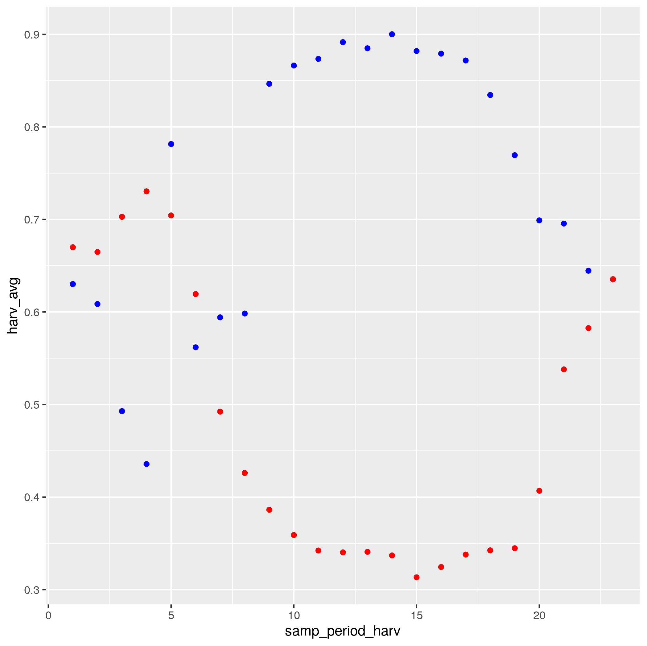
1. Plot the whole-raster mean NDVI (cellStats()) for Harvard Forest and SJER through time using different colors for the two sites. To do this:
   • Load the files for each site as a raster stack
   • Use cellStats() to calculate the mean values for each raster in the stack. Call the outputs harv_avg and sjer_avg
   • Create a vector of sampling periods for each site: e.g., samp_period_harv = 1:length(harv_avg)
   • Make a data frame that includes the sampling period column and the average NDVI values
   • Make a plot with NDVI on the y axis and sampling period on the x axis. Since you have two different data frames you’ll need to include each data frame in a different geom_point layer.
2. Extract the NDVI values from all rasters for the HARV_plots and sjer_plotsin neon-airborne/plot_locations. Running extract() on a raster stack results in a matrix with one column per raster and one row per point. To more easily work with this data, we want to have one column with the raster names and one column per point, which you can do by transposing the matrix with the t() function. Do this for both HARV and SJER.

Expected outputs for Phenology from Space